CountBio
Mathematical tools for natural sciences
Basic Statistics with R
The F distribution
The F distribution arises when we compare the variances of two normal distributions by taking their ratio.
Suppose we draw random samples of sizes \(\small{n_1}\) and \(\small{n_2}\) from two normal distributions \(\small{N(\mu_1, \sigma_1^2) }\) and \(\small{N(\mu_2, \sigma_2^2) }\) respectively. Let \(\small{s_1^2 }\) and \(\small{s_2^2 }\) be the estimated variances of these two data sets.
For these two sets of observations, the ratio of sample to the population variances is written as \(\small{\dfrac{s_1^2}{\sigma_1^2} }\) and \(\small{\dfrac{s_2^2}{\sigma_2^2} }\).
We define a new variable F which is the ratio of these two ratios. We then manipulate this expressions to define two new variables U and V:
Computation of probabilities from F distribution
Similar to what we did with the Gaussian distribution, we can compute the probability of getting more than or less than certain value of F statistic. See the figure below:
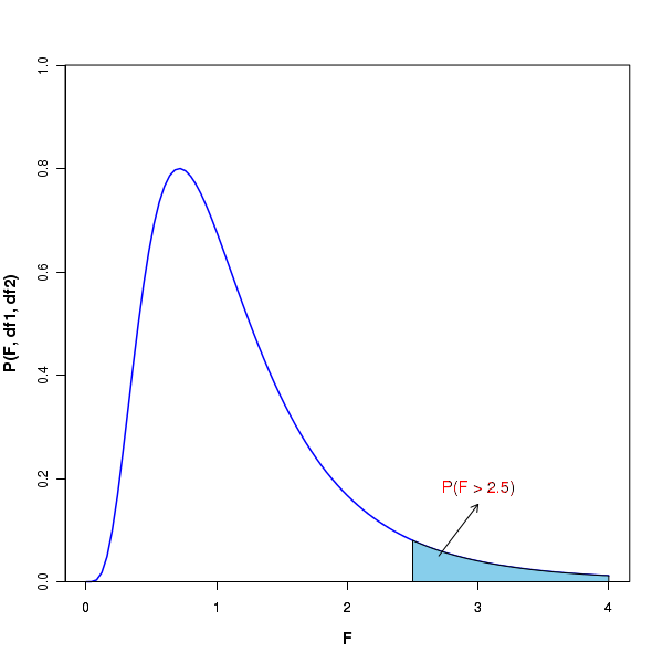
In the above figure, the plot at the top shows the shaded area which represent the probabilities above a particular \(\small{F}\) value. In an F distribution with given degrees of freedom df1 and df2, there is a p-value corresponding to every F value that represents the area under the curve above that F. The p value is computed for a given $F(df_1, df_2)$ with two degrees of freedom. One such F-distribution table can be accessed from here. In this table, the \(\small{F}\) values corresponding to \(\small{\alpha = 0.05, 0.1 and 0.01\) are tabulated for many pairs of degrees of freedom (df1, df2) for certain discrete values in the range of 1 to 100. Look at the the table corrsponding to p=0.05, for example. Corresponding to a degrees of freedom \(\small{df1=n-1=10}\) and \(\small{df2=n-2=10 }\), the p-value of 0.05 represents the area undet the F curve above F=2.9782. Similarly, let us look at the table corresponding to p=0.01. For the degrees of freedom \(\small{ df1=9}\) and \(\small{df2 = 30 }\), the p-value of 0.01 represents the area under the curve above F=3.067. We can write the above statements as, \(~~~~~~~~~~~~~\small{F_{0.05}(df1=10, df2=10) = 2.9782} \) and, \(~~~~~\small{F_{0.01}(df1=9, df2=30) = 3.067} \) To get a p-value for any value of F statistic from the distribution F(df1, df2), R provides a function \(~~\small{pf(F, df1, df2)}\) which returns the area under the F diatribution from \(\small{F = 0~to~t}\) for given degrees of freedom \(\small{df1, df2}\). We should subtract this value from 1 to get the area under the curve from F to infinity.
Now we will learn to use the R library functions for the t distribution.
R scripts
Let F = F distribution variblen = sample sizer1 = n1-1, r2 = n2-1 = degrees of freedom Then,df(F, r1, r2) -----> returns the probability density at t on a F distribution curve with degrees of freedom r1, r2.rf(m, r1, r2) -----> returns m random deviates from r distribution with r1 and r2 degrees of freedomqf(p, r1, r2) -----> returns the F value corresponding to a cumulative probability p on a F distribtuion with r1 and f2 degrees of freedom.pf(F, r1, r2) -----> returns the cumulative probability p from minus infinity to F on a F distribution with r1 and r2 degrees of freedom.
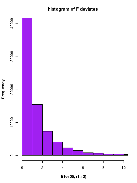
##### Using R library functions for the F distribution

#### probability density function
n1 = 10
n2 = 12
r1 = n1-1
r2 = n2-2
F = 2.5

F_density = df(F, r1, r2)
F_density = round(F_density, digits=2)
print(paste("probability density for F = ", F, " and degree of freedom = ", r1,"
              and ", r2, " is ", F_density))

### Generating the curve of F distribution probability density

x = seq(0,5,0.1)

r1 = 10
r2 = 12

string = "P(F,r1=10, r2=12)"

curve(df(x, r1, r2), xlim=c(0,4), xlab="F", ylab=string, lwd=1.5, cex.lab=1.2, col="blue",
                     main="F distribution", font.lab=2)


#### Generating cumulative probability (p-value) above upto a F value in a F distribution

#######  pf(F, r1, r2) generates cumulative probability from 0 to given F value.
#######  The probability of having a value above F is 1 - pf(F, r1, r2)

r1 = 10
r2 = 12

F = 2.8
pvalue = pf(F, r1, r2)
pvalue = round(pvalue,3)
print(paste("cumulative probability from F = 0 to ", F, "is ", pvalue))


#### Generating F value for which the cumulative probability from 0 to F is p.
###  The function qf(p,r1, r2) returns F value at which cumulative probability is p.

p = 0.95  ## cumulative probabilitu from 0 to F.
F = qf(p, r1, r2)
F = round(F, digits=3)
print(paste("F value for a cumulative probability p = ", p, "is ", F))


#### Generating random deviates from a t distribution
### rf(m, f1, f2) returns a vector of m random deviates from a F of given F(r1,r2)

r1 = 10
r2 = 12
ndev = rf(4, r1, r2)
ndev = round(ndev,digits=3)
print("Four random deviates from F distribution with (10, 12) degrees of freedom : ")
print(ndev)

X11()

## plotting the histogram of 100000 random deviates from unit Gaussian:
r1 = 10
r2 = 12
hist(rf(100000, r1, r2), breaks=60, xlim = c(0,10), ylim = c(0, 25000), col="purple",
        main="histogram of F deviates", font.lab=2)
Executing the above script in R prints the following results and figures of probability distribution on the screen:
[1] "probability density for F =  2.5  and degree of freedom =  9  and  10  is  0.09"
[1] "cumulative probability from F = 0 to  2.8 is  0.953"
[1] "F value for a cumulative probability p =  0.95 is  2.753"
[1] "Four random deviates from F distribution with (10, 12) degrees of freedom : "
[1] 1.157 0.169 0.787 1.044