CountBio
Mathematical tools for natural sciences
Basic Statistics with R
Binomial distribution
The bionomial distribution is a discrete probability distribution of the number of successes observed in a fixed number of Bernoulli trials. Suppose our experiment involves tossing 10 coins and noting down the number of heads(success). First time, we tossed 10 coins and observed 3 heads (and 7 tails). This is same as performing a sequence of 10 Bernoulli trials , each with a probability of success \( \small{ p = \frac{1}{2}} \). We repeat this experiment large number of times, noting down the number of heads \(x\) we get everytime we toss 10 coins. We will end up with a set of values like,
\( x = \{3,5,8,1,4,9,10,2,5,7,4,5,3,8,9.....\} \). The number of successes x out of 10 trials in the above data set varies from 0 (no head observed amont the 10 coins tossed, all are tails) to a maximum of 10 (all 10 coins showed head). The discrete probability distribution of \(x\) is a binomial distribution.
The binomial distribution is a discrete probability distribution of \(x\) successes in a sequence of \(n\) Bernoulli trials, each with a probability of success \(p\).
A sequence of experiments can be treated as a binomial process if they have the following properties:
- There should be a finite number of trials n
- The \(n\) trials are considered to be independent of each other
- Each trial should have only two mutually exclusive outcomes
- The probability of success \(p\) remains same from trial to trial
Derivation of binomial probability: Let \(x\) be the number of successes in n Bernoulli trials with probability of success \(p\) and probability of failure \(q = 1-p \). The possible values of \(x\) are \(0,1,2,3,...n\). Remember that if \(x\) successes occur, then \(n-x\) failures will occur. Since any \(x\) trials among \(n\) can result in a success, we have to compute the number of ways in which we can choose \(x\) trials out of \(n\) trials for assigning success. This is same as choosing \(x\) objects out of \(n\) in \(_nC_x\) possible ways without worrying about ordering the \(x\) objects. Therefore,the number of ways of selecting positions for \(x\) successes in a sequence of \(n\) trials is,
\(\small{_nC_x = \dfrac{n!}{x!(n-x)!} }\)Since the trials are independent of each other,
probability of \(x\) successes = \(p \times p \times p \times....(x~times) \) = \(\small{ p^x }\)
probability of (n-x) failures = \((1-p) \times (1-p) \times (1-p) \times.....(n-x~~times) \) = \( \small{(1-p)^{n-x} }\)
Therefore, the probability of getting \(x\) successes and \(n-x\) failures in \(n\) Bernoulli trials = \(\small{ p^x (1-p)^{n-x}}\)
Since \(x\) successes and \(n-x\) failures can happen in \(\small{ \dfrac{n!}{x!(n-x)!}} \) mutually exclusive ways, we have to sum the probability \(\small{ p^x (1-p)^{n-x}}\) over \( \small{ \dfrac{n!}{x!(n-x)!}} \), which is equivalent to multiplying the two expressions:
\(\small{P_b(x,n,p) = \dfrac{n!}{x!(n-x)!} p^x (1-p)^{n-x}~~~~~~~with~~x=0,1,2,3,4,....n }\)Therefore, the binomial probability of getting \(x\) successes in a sequence of \(n\) Bernoulli trials, where \(p\) is the probability of success in a single trial is given by,
The terms \(n\) and \(p\) are called the parameters of the binomial distribution.
Why it is called "binomial" distribution?
According to Binomial theorem, if \(p\) and \(q\) are two variables representing real numbers, then the expansion \((p+q)^x \) for an integer \(x\) can be written as,
\(\small{(p + q)^n = p^n + n p^{n-1} q + n(n-1)p^{n-2}q^2 + ....+ x^n = \sum\limits_{x=0}^n \dfrac{n!}{x!(n-x)!} p^x q^{n-x} }\)
Comparing the above expression with the binomial probability formula, we realize that for \(q=1-p\), the binomial probability expression is of the same form as the successive terms of a binomial expansion. hnce the name "binomial distribution".
Mean and variance of the binomial distribution
Once we have established the mathematical expression for the binomial probability distribution \(P_b(x,n,p)\), we can get an expression for the population mean \(\mu\) and variance \(\sigma^2\) using the first and second moments of the distribution. We state the results here without full derivation:
\(\small{\mu = \sum\limits_{x=0}^n x P_b(x,n,p) = \sum\limits_{x=0}^n x \dfrac{n!}{x!(n-x)!} p^x (1-p)^{n-x} = np } \) \(\small{\sigma^2 = \sum\limits_{x=0}^n (x-\mu)^2P_b(x,n,p) = \sum\limits_{x=0}^n (x - np)^2 \dfrac{n!}{x!(n-x)!} p^x (1-p)^{n-x} = np(1-p) } \)
We must understand that the above mentioned quantities are the mean and variance of the population following bionomial distribution with a given \(n\) and \(p\). These are expected values. If we repeat the experiment finite number of times, the observed mean and variance will deviate from the expected values.
We summarize the formulas of binomial probability distribution:
From the above expressions for mean \(\mu\) and \(\sigma^2\), we realize that \(\small{\sigma^2 = np(1-p) = \mu(1-p) }\).
The plot of binomial probability distribution
The discrete probability values \(P_b(x,n,p)\) have been plotted for various x values in the figure below:
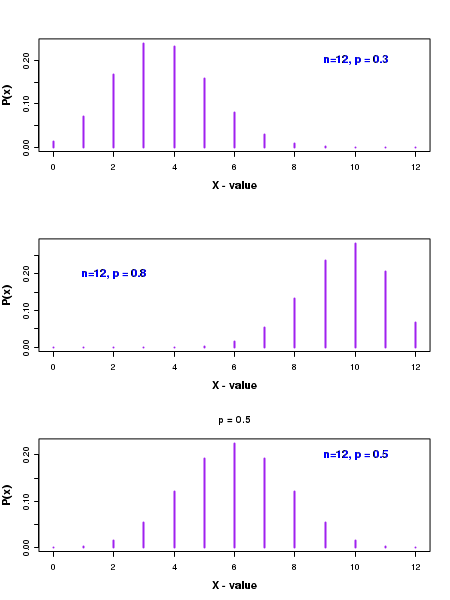
In the above figure, we can notice that the shape of the distribution is decided by the probability \(p\) for success in a single trial. When the value of \(p\) is less than 0.5, the distribution is skewed to the left, as seen in top figure corresponding to a value of \(\small{p=0.3}\).
On the other hand, when \(p\) is greater than 0.5, the distribution is skewed to the right, as seen in the second figure from top corresponding to \(\small{p=0.8 }\).
When the probabuility p is exactly 0.5, the distribution is symmetric about its mean value of \( \small{np = 12\times0.5=6 }\), as shown in third figure from top.
We will now learn to compute binomial probability distribution in R
R scripts
We perform various computations on binomial distribution using the inbuilt library functions in R.
The R statistics library provides the following four basic functions for the binomial distribution. In fact, similar set of 4 functions are provided for every distribution in R.
Let x be the number of successes inn Bernoulli trials, each with a probability of successp .dbinom(x,n,p) -----> Returns the binomial probability of getting a valuex . This is called "probability density".pbinom(x,n,p) -----> Returns the cumulative probability of this binomial distribution from x=0 to given x. Thus, qbinom(x=2,n,p) = qbinom(0,n,p)+qbinom(1,n,p)+qbinom(2,n,p)qbinom(x,n,p) -----> Inverse of the pbinom() function. Returns the x value upto which the cumulative probability is p (quantiles).rbinom(m,n,p) -----> Returns m "random deviates" from a binomial distribution of (n,p). Each one of the random deviate is the number of successes x observed in n trials, with p being probability of success in a single trial.
The usage of these four functions are demonstrated in the R script here. With comments, the script lines are self explanatory:
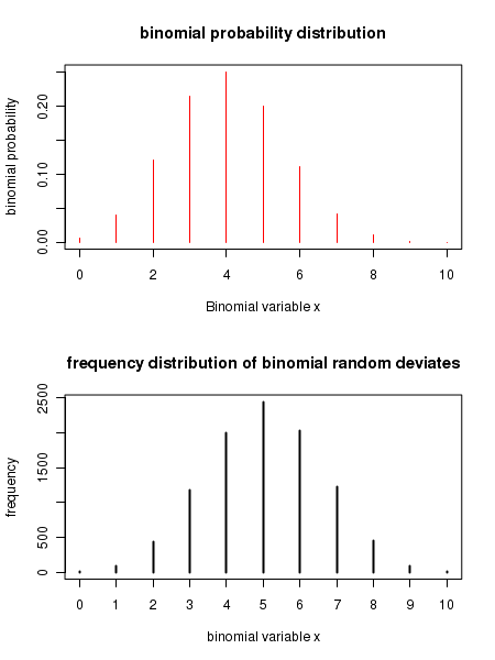
##### Using R library functions for binomial distribution

n = 10   ## number of trials
p = 0.5  ## probability of success in a trial
x = 3    ## number of successes


### Probability density function.
### dbinom(x,n,p) returns the binomial probability for x successes in n trials, where p is probability
###    of success in a single trial
binomial_probability = dbinom(x,n,p)
print(paste("binomial probability for (",x,",",n,",",p,") = ",binomial_probability) )


### Function for computing cumulative probability.
### pbinom(x,n,p) gives cumulative probability for a binomial distribution from 0 to x.
cumulative_probability = pbinom(x,n,p)
print(paste("cumulative binomial probability for (",x,",",n,",",p,") = ",cumulative_probability) )


### Function for finding x value corresponing to a cumulative probability
x_value = qbinom(cumulative_probability, n, p)
print(paste("x value corresponding to the given  cumulative binomial probability = ",x_value) )

### Function that returns 4 random deviates from a Binomial distribution of given (n,p)
deviates = rbinom(4, n, p)
print(paste("4 binomial deviates :  "))
print(deviates)

par(mfrow = c(2,1))

### We plot a binomial density distribution using dbinom()
n = 10
p = 0.4
x = seq(0,10)
pdens = dbinom(x,n,p)
plot(x,pdens, type="h", col="red", xlab = "Binomial variable x", ylab="binomial probability",
       main="binomial probability distribution")


## We generate frequency histogram of binomial deviates using rbinom()
n = 10
p = 0.5
xdev= rbinom(10000, n, p)
plot(table(xdev), type="h", xlab="binomial variable x", ylab="frequency",
            main="frequency distribution of binomial random deviates")
Executing the above script in R prints the following results and figures of probability distribution on the screen:
[1] "binomial probability for ( 3 , 10 , 0.5 ) =  0.1171875"
[1] "cumulative binomial probability for ( 3 , 10 , 0.5 ) =  0.171875"
[1] "x value corresponding to the given  cumulative binomial probability =  3"
[1] "4 binomial deviates :  "
[1] 6 6 8 4