CountBio
Mathematical tools for natural sciences
Basic Statistics with R
Linear Regression
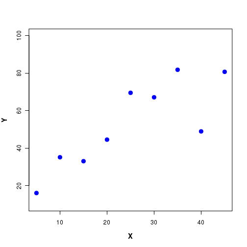
In order to establish the relationship between two variables X and Y, we perform experiments. We treat one of the variables (say X) as an independent variable and measure the values of Y for various values of X. The variable Y is called a dependent variable , since it is measured for a set of fixed values of X. The independent variable X is also called the predictor variable and Y the response variable . A set of data points between X and Y are shown in Figure-1 below:
By looking at the scatterplot, suppose we decide that the relationship between X and Y can be approximated to be linear . We want to approximate the data points by a stright line of the form $y = a + bx$ so that for any given value of x in the data range, we can easily compute the approximate value of y from this equation. This is called a linear model for this data set.
By constructing this linear model, we replace a set of data points by the equation of a stright line through the points which approximately describes the relationship between X and Y in the given range of data. This helps us to qualitatively and quantitatively understand such a variation. Once the linear relationship is established, we can examine the inherent phenomena that result in a linear variation of Y as a function of X.
The problem is that infinite number of stright lines, each with a distinct slope and intercept, can pass through the given set of points. Three such lines are depicted in Figure-2 here:
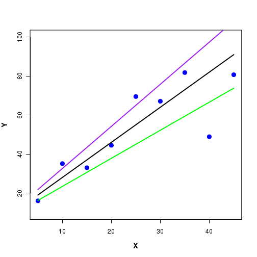
In the above Figure-2 we notice that each one of the three lines through the data lie close to some points and far away from sone other points. Which one is the best one?
The method of linear regression uses the observed data points to compute the slope and the intercept of the best straight line that can pass through the data points. The mathematical method is called the least square fit to a straight line . A straight line obtained from the observed data points (X,Y) using least square fit has the least deviation (error) between expected Y value on the line and the experimentally observed Y value for a given X value, when compared to any other line through the data points.
Important point : The method of least square fit to a stright line (linear regression) gives the best straight line through the data, with error minimized compared to any other line. It does not mean that such a line is the best curve through the data points. For example, for a given set of data points, the line obtained from least square method may have more error(deviations) from data points when compared to a polinomial of 5th degree obtained from least square fit of data to a polinomial!. Having decided to fit a curve (line strightline, exponential, polinomial etc) through the data point, the least square method gives the best curve (that minimized the error) in the family. If we decided to fit a strightline, we get the best stright line. If we decide to fit a parabola, we get the best parabola. Thus, for a given curve, the method of least squares gets the best parameters of the curve. If \(\small{y = mx+c}\) is the curve fitted, the method gives the best values for m and c that minimizes the error. Similarly, if \(\small{y = a_0 + a_1x^2 + a_2x^3 + a_3x^4}\) is the fitted curve, the method gives the best values for the coefficients \(\small{a_0, a_1, a_2, a_3 and a_4}\) that minimized the error.
Before going into the procedure, we will list the assumptions underlying the liear regression:
Suppose, we denote the data points as ($x_1,y_1$), ($x_2,y_2$), ($x_3,y_3$), ...., ($x_n,y_n$).
1. The values of the independent variable X are fixed, and have no errors. X is a non-random variable.2. For a given value of X, the possible Y values are randomly drawn from a sub population of normal distribution. Thus, for a given value $x_i$ of X, observed $y_i$ is a point randomly drawn from a normal distribution. Also, the Y values for different X values are independent.
3. The means of the parent normal distributions from which the points $y_1, y_2,...,y_n$ were drawn lie on a straight line. The linear regression method in fact computes the slope and intercept of the straight line.. This can be expressed as an equation, $$ \mu_{y,x} = \beta_0 + \beta_1x$$ where $\mu_{y,x}$ is the mean value of the population from which the point y was drawn for the given x value. The coefficients $\beta_0$ and $\beta_1$ are called regression coefficients . 4. The variances of the parent normal distributions to which $y_1, y_2, ..., y_n$ belong can be assumed to be either equal or not equal in the derivation. Different expression will result based on these two assumptions. Regression analysis procedure
For the given data set (X,Y), let $y = \beta_0 + \beta_1x$ be the regression equation we want.
Since the we will never know the true regression coefficients, we will make an estimate of these coefficients from the data points. We name them $b_0$ and $b_1$ respectivly so that $y = b_0+b_1 x$ for the observed data set.
For a given $x_i$, let the observed Y value be $y_i$. Then, $P_{obs}(x_i, y_i)$ will be this observed data point.
For a given $x_i$ value, let $y_i^{r}$ denote the corresponding point on this regression line. Then $P_{exp}(x_i, y_i)$ will be the expected data point on the regression line. See the Fifure-3 below:
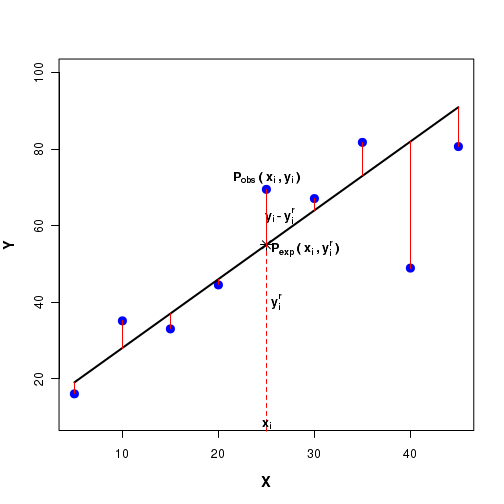
The linear regression procedure computes the square of the difference $(y_i - y_i^r)^2$ between the observed $y_i$ value and the expected $y_i^r$ value on the line for each data point. Using a minimization procudre, the sum of the squares of the differences $\sum(y_i - y_i^r)^2$ are minimized to get the coefficients $b_0$ and $b_1$.
For a given $x_i$, we have $y_i^r = b_0 + b_1x_i$. Using this, we can write the sum square as,
$$ \chi^2 = \sum_{i}\dfrac{1}{\sigma_i^2}(y_i - (b_0 + b_1 x_i) )^2$$By minimizing the above mentioned $\chi^2$ expression with respect to variables $b_0$ and $b_1$, we can get expressions for $b_0$ and $b_1$ in terms of observed data points ($x_i, y_i$). Using them we can compute $y_i = b_0 + b_1 x_i$ to plot the straight line through the data points.
See the box below for a complete derivation.
In the derivation, we consider two cases. The observed value $y_i$ is assumed to be a random sample derived from a Normal distribution $N(\mu_i, \sigma_i)$. In the first case, we assume that the standard deviations $\sigma_i$ are all equal. That is, all data points are drawn from distributions whose variances $\sigma_i$ are equal. In the second case, we assume that these variances $\sigma_i$ are unequal.
Derivation of linear regression coefficients: We start with our basic assumption that for a given independent variable $x_i$, the observed value $y_i$ follows a gaussian with mean $\mu_i = y(x_i) = b_0 + b_1x$ and standard deviation $\sigma_i$. For each point $(x_i, y_i)$, we write the Gaussian probability density as, \( ~~~~~~~~~~~~~~~\small{P_i(x_i,y_i) = \dfrac{1}{\sigma_i \sqrt{2\pi}} {\Large e}^{-\dfrac{1}{2}\left(\dfrac{y_i-y(x_i)}{\sigma_i}\right)^2} }\) The probability of observing n such independent data points is obtained by multiplying their individual probabilities: \(\small{P(data~set~with~n~points) = P(x_1,y_1) \times P(x_2,y_2) \times P(x_3,y_3) \times .....\times P(x_n,y_n) }\) \(~~~~~~~~~~~~~~~~~~~~~~~~~~~~~~~~~~~~\small{= \displaystyle\prod_{i=1}^{n} P(x_i,y_i) }\) \(~~~~~~~~~~~~~~~~~~~~~~~~~~~~~~~~~~~~\small{= \displaystyle\prod_{i=1}^{n} \dfrac{1}{\sigma_i\sqrt{2\pi}} {\Large e}^{-\dfrac{1}{2} \left(\dfrac{y_i-y(x_i)}{\sigma_i} \right)^2 } }\) \(~~~~~~~~~~~~~~~~~~~~~~~~~~~~~~~~~~~~\small{= \displaystyle\prod_{i=1}^{n} \dfrac{1}{\sigma_i\sqrt{2\pi}} {\Large e}^{-\dfrac{1}{2} \left(\dfrac{y_i-(b_0+b_1x_i)}{\sigma_i} \right)^2 } }\) Since the multiplication of exponential terms is equivalent to summing their exponents, we can write the above expression as, \(~~~~~~\small{ P(data~set~with~n~points)~=~\displaystyle{\left( \prod_{i=1}^{n} \dfrac{1}{\sigma_i\sqrt{2\pi}}\right)} ~ {\Large e}^{-\dfrac{1}{2} \displaystyle \sum_{i=1}^{n} \left( \dfrac{y_i-(b_0+b_1x_i)}{\sigma_i} \right)^2 } } \) The best values of $b_0$ and $b_1$ are the ones for which the above probability of data set is maximum . By looking at the expression we can realize that the probability is maximum when the negative exponent term given by, \(~~~~~~~~~~~~~~~~\small{\chi^2~=~\displaystyle\sum_{i=1}^{n} \dfrac{1}{\sigma_i^2} \left(y_i - b_0 - b_1x_i)^2 \right) }~~~~~~~\)is a minimum. The above term is called The least square sum . We have a data set with n date points (x_i, y_i) in which each $y_i$ is assumed to be randomly drawn from a Gaussian with mean $y(x_i) = b_0+b_1x_i$ and standard deviation $\sigma_i$. By minimizing the above least square sum with respect to the variable $b_0$ and $b_1$, we can obtain their best values for the data set. The line $y(x_i) = b_0 + b_1x_i$ is said to be the best fit to the data which minimizes the errors between observed $y_i$ values and the expected values $y(x_i)$ on the straight line. This procedure is also called as a least square fot to a straight line. The best fit valus for $b_0$ and $b_1$ are obtained by solving the equaltions, \( \dfrac{\partial \chi^2}{\partial b_0} = 0~~~~~~~~~and~~~~~~~ \dfrac{\partial \chi^2}{\partial b_1} = 0 \) At this stage, we consider two cases related to our assumption regarding the standard deviations:
Case 1 : The standard deviations $\sigma_i$ are all equal
We take the case for which \(\small{\sigma_1 = \sigma_2 = .....= \sigma_i = \sigma }\)
The expression for \(\small{\chi^2 }\) becomes,
\(~~~~~~\small{\chi^2 = \displaystyle\sum_{i=1}^{n} \dfrac{1}{\sigma^2}(y_i - b_0 - b_1x_i)^2 }\)
\(~~~~~~\small{~~~~= \dfrac{1}{\sigma^2}\displaystyle\sum_{i=1}^{n} (y_i - b_0 - b_1x_i)^2 }\)
Differentiating \(\small{\chi^2 }\) partially with respect to $b_0$ and $b_1$ and equating to zero, we get two equations:
\(\small{\dfrac{\partial \chi^2}{\partial b_0}~~=~~ \dfrac{-2}{\sigma^2} \displaystyle\sum_{i=1}^{n} (y_i - b_0 - b_1x_i)~~=~~0 }~~~~~~~~~~~~(1)\)
\(\small{\dfrac{\partial \chi^2}{\partial b_0}~~=~~ \dfrac{-2}{\sigma^2} \displaystyle\sum_{i=1}^{n} (y_i - b_0 - b_1x_i) x_i~~=~~0 }~~~~~~~~~~~~(2)\)
Equations (1) and (2) can be rearranged to get the following two simultaneous equations with $b_0$ and $b_1$ as variables:
\(\small{ \displaystyle\sum_{i=1}^{n} y_i~=~\displaystyle\sum_{i=1}^{n} b_0~+~\displaystyle\sum_{i=1}^{n} b_1x_i~=~ b_0n~+~b_1\displaystyle\sum_{i=1}^{n}x_i }~~~~~~~~(3)\)
\(\small{ \displaystyle\sum_{i=1}^{n}x_iy_i~=~ \displaystyle\sum_{i=1}^{n}b_0x_i~+~ \displaystyle\sum_{i=1}^{n} b_1 x_i^2~~=~~ b_0 \displaystyle\sum_{i=1}^{n}x_i~+~b_1 \displaystyle\sum_{i=1}^{n}x_i^2 }~~~~~~~~~~~~(4)\)
Solving the equations (3) and (4) for the variables $b_0$ and $b_1$, we get the following expressions for the coefficients of the least square fit for the case when all the data points have equal veriances. All the summations are over the index $i=1~to~n$, where n is the number of data points.
\(\small{
\Delta~=~
\begin{vmatrix}
n & \displaystyle\sum x_i \\
\displaystyle\sum x_i & \displaystyle\sum x_i^2 \\
\end{vmatrix}
~~=~~n \sum x_i^2 - (\sum x_i)^2
}\)
\(\small{
b_0~=~\dfrac{1}{\Delta}
\begin{vmatrix}
\displaystyle\sum y_i & \displaystyle\sum x_i \\
\displaystyle\sum x_i y_i & \displaystyle\sum x_i^2 \\
\end{vmatrix}
~~=~~\dfrac{1}{\Delta} \left(\sum y_i \sum x_i^2 - \sum x_i \sum x_i y_i\right)
}\)
\(\small{
b_1~=~\dfrac{1}{\Delta}
\begin{vmatrix}
n & \displaystyle\sum y_i \\
\displaystyle\sum x_i & \displaystyle\sum x_i y_i \\
\end{vmatrix}
~~=~~\dfrac{1}{\Delta} \left(n \sum x_i y_i - \sum x_i \sum y_i \right)
}\)
Case 2 : The standard deviations $\sigma_i$ are unequal
In this case, the standard deviations of populations from which $y_i$ were drawn are not equal. As a consequence, we cannot pull out the standard deviation term $\sigma_i$ out of the summations. We will go back to the derivation where we defined the Chi-square term:
\(~~~~~~~~~~~~~~~~\small{\chi^2~=~\displaystyle\sum_{i=1}^{n} \dfrac{1}{\sigma_i^2} \left(y_i - b_0 - b_1x_i)^2 \right) }~~~~~~~\) Now, differentiating with respect to the variables $b_0$ and $b_1$, we get \(\small{\dfrac{\partial \chi^2}{\partial b_0}~~=~~ -2 \displaystyle\sum_{i=1}^{n} \dfrac{1}{\sigma_i^2} (y_i - b_0 - b_1x_i)~~=~~0 }~~~~~~~~~~~~(5)\) \(\small{\dfrac{\partial \chi^2}{\partial b_1}~~=~~ -2\displaystyle\sum_{i=1}^{n} \dfrac{1}{\sigma_i^2}(y_i - b_0 - b_1x_i) x_i~~=~~0 }~~~~~~~~~~~~(6)\) Equations (5) and (6) can be rearranged to get the following two simultaneous equations with $b_0$ and $b_1$ as variables: \(\small{ \displaystyle\sum_{i=1}^{n} \dfrac{y_i}{\sigma_i^2}~=~ b_0 \sum \dfrac{1}{\sigma_i^2}~+~b_1\displaystyle\sum_{i=1}^{n} \dfrac{x_i}{\sigma_i^2} } ~~~~~~~~(7)\) \(\small{ \displaystyle\sum_{i=1}^{n} \dfrac{x_iy_i}{\sigma_i^2 }~=~ b_0 \displaystyle\sum_{i=1}^{n} \dfrac{x_i}{\sigma_i^2}~+~b_1 \displaystyle\sum_{i=1}^{n} \dfrac{x_i^2}{\sigma_i^2} }~~~~~~~~~~~~(8)\) Solving the above two equations for the variables $b_0$ and $b_1$, we get their expressions in terms of the data points $(x_i, y_i$ : \(\small{ \Delta~=~ \begin{vmatrix} \displaystyle\sum\dfrac{1}{\sigma_i^2} & \displaystyle\sum\dfrac{x_i}{\sigma_i^2} \\ \displaystyle\sum\dfrac{x_i}{\sigma_i^2} & \displaystyle\sum\dfrac{x_i^2}{\sigma_i^2} \\ \end{vmatrix} ~~=~~\displaystyle\sum\dfrac{1}{\sigma_i^2} \sum\dfrac{x_i^2}{\sigma_i^2} - \displaystyle\sum\dfrac{x_i}{\sigma_i^2} \sum\dfrac{x_i}{\sigma_i^2} }\) \(\small{ b_0~=~\dfrac{1}{\Delta} \begin{vmatrix} \displaystyle\sum \dfrac{y_i}{\sigma_i^2} & \displaystyle\sum \dfrac{x_i}{\sigma_i^2} \\ \displaystyle\sum \dfrac{x_i y_i}{\sigma_i^2} & \displaystyle\sum \dfrac{x_i^2}{\sigma_i^2} \\ \end{vmatrix} ~~=~~\dfrac{1}{\Delta} \left(\sum \dfrac{y_i}{\sigma_i^2} \sum \dfrac{x_i^2}{\sigma_i^2} - \sum \dfrac{x_i}{\sigma_i^2} \sum \dfrac{x_i y_i}{\sigma_i^2}\right) }\) \(\small{ b_1~=~\dfrac{1}{\Delta} \begin{vmatrix} \displaystyle\sum\dfrac{1}{\sigma_i^2} & \displaystyle\sum \dfrac{y_i}{\sigma_i^2} \\ \displaystyle\sum \dfrac{x_i}{\sigma_i^2} & \displaystyle\sum \dfrac{x_i y_i}{\sigma_i^2} \\ \end{vmatrix} ~~=~~\dfrac{1}{\Delta}\left(\displaystyle\sum\dfrac{1}{\sigma_i^2} \displaystyle\sum \dfrac{x_i y_i}{\sigma_i^2}~~-~~\displaystyle\sum \dfrac{x_i}{\sigma_i^2} \displaystyle\sum \dfrac{y_i}{\sigma_i^2}\right) }\) Evaluating the quality of the fit
From the data points, we have obtained the regression coefficients. The question is, how good is this regression line for describing the relationship between X and Y variables?
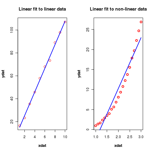
For exmaple, suppose we have (wrongly) decided to fit a straight line to a data that follows a parabolic relationship between X and Y. We also got a regression equation. In this case, though the regression line is the best fit possible to the data, it may not correctly represent the relationship between the variables. Figure-4 below illustrates this:
In order to decide whether the regression equation reasonably represents the trend in the data, certain statistical tests can be performed. We will consider some of them here.
The coefficient of determination, $r^2$
To obtain a number that represents the quality of the fit, we compare the scateering of the data points about the fitted line with their scateering around their mean value $\overline{y}$
In the Figure-5 below, the blue line is the regression line through the data points represented by red circles. The location of horizontal black line shows the mean of y values of data points.
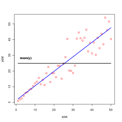
Let us consider the following quantities obtained from the data: $x_i$ = the x values of data points $y_i$ = the y values of the data points $y(x_i) = b_0 + b_1 x_i$ = the value on the fitted line for a $x_i$ $\overline{y}$ = the mean of all the $y_i$ values of data points
We can write the difference $(y_i - \overline{y})$ as,
$$ (y_i - \overline{y})~~=~~(y(x_i) - \overline{y})~~+~~(y_i - \hat{y_i}) $$The three terms can be understood as follows:
$(y_i - \overline{y})$ is the vertical distance of of an observed value from the mean value. This is called the total deviation
$(y(x_i) - \overline{y})$ is the vertical distance of mean value of data point from the fitted line. This is called the explained deviation. Explains the reduction in deviation because of fitting.
$(y_i - y(x_i))$ is the vertical distance of a data point from the mean vertical distance. This is called the unexplained deviation. Remains 'unexpalined' even after fitting the line.
We can write the following equation with their sum of squares:
$$ \sum_i{(y_i - \overline{y})^2}~~=~~\sum_i{(y(x_i) - \overline{y})^2}~~+~~\sum_i{(y_i - y(x_i))^2} $$
with the following names,
$\sum{(y_i - \overline{y})^2}$ = SST = Total sum of squares
$\sum{(y(x_i) - \overline{y})^2}$ = SSR = Explained sum of squares
$\sum{(y_i - y(x_i))^2}$ = SSE Unexplained sum of squares.
Using the above mentioned parameters from data, we will now deduce an expression for the quality of fit.
Suppose the fit is very good so that the data points are close to the fitted line.
In this case, the value of the explained sum of squares $\sum{(y(x_i) - \overline{y})^2}$ will constitute a large fraction of the total sum of squares $\sum{(y_i - \overline{y})^2}$. Hence the ratio $\frac{SSR}{SST}$ will be close to 1.
Suppose the data points are scattered all over resulting in a very bad fit.
In this case, the (explained) sum square deviations from the mean $\sum{(y(x_i) - \overline{y})^2}$ will be a smaller fraction of the total sum of squares $\sum{(y_i - \overline{y})^2}$. Hence the ratio $\frac{SSR}{SST}$ will be close to 0.
Based on these arguments, the coefficient of determination $r^2$ is defined as,
$$ r^2 = \frac{\sum{(y(x_i) - \overline{y})^2} }{\sum{(y_i - \overline{y})^2}} = \frac{SSR}{SST}$$As $r^2 \rightarrow 1$, the fit gets better and better. When the data points perfectly lie on a straight line, $r = 1$.
As $r^2 \rightarrow 0$, the fit gets worse and worse. When the data points are perfectly random, $r = 0$.
Statistical tests for the parameter estimation
In the regression analysis, the estimated parameters $\beta_0$ and $\beta_1$ are the unbiased point estimators of the corresponding parameters $b_0$ and $b_1$. We can conduct hypothesis tests like t-test, F-test and ANOVA on the regression coefficients.
The t-test
For a chosen value of $b_1'$, we test the null hypothesis that $b_1 = b_1'$ against an alternate hypothesis that they are not equal with a t statistic. ie.,
$$ H_0 : b_1 = b_1' $$ $$ H_A : b_1 \neq b_1' $$Note : When $b_1' = 0$, we test the null hypothesis $ H_0 : b_1 = 0 $
The t-statistic for this test is defined as,
$$ T = \frac{b_1 - b_1'}{S_{b_1}}$$where Mean Standard Error (MSE) $S_{b_1}$ is computed from the expression,
$$ S_{b_1} = \sqrt{ \frac{ \frac{\sum{(y_i - y(x_i))^2}}{n-2} } {\sum{(x_i - \overline{x})^2}} } $$The computed statistic T follows a t-distribution with $n-2$ degrees of freedom, where $n$ is the number of observations.
For a pre-decided critical value $\alpha$, the null hypothesis accepted if the test statistic T lies within the critical region,
$$ -t_{\alpha/2}(n-2) \lt T \lt t_{\alpha/2}(n-2)$$where $t_{\alpha/2}(n-2)$ is the percentile of the t distribution with n-2 degrees of freedom corresponding to a cumulative probability of $1-\alpha/2$.
The $100(1-\alpha)$ percent confidence interval for the estimated $\hat{\beta_1}$ is given by,
$$ b_1 \pm t_{\alpha/2, n-2} S_{b_1} $$The statistical significance or the p-value for the test is defined as
$$ p = 2 \times P(t \geq T) $$A similar t-test can be performed to test the null hypothesis $b_0 = b_0'$ for the intercept.
The appropriate T statistics is expressed as,
$$ T = \frac{b_0 - b_0'}{S_{b_0}} $$Where
$$ {S_{b_0}} = \sqrt{\frac{\sum(y_i - y(x_i))^2}{n-2} [\frac{1}{n} + \frac{\overline{x}^2}{\sum(x_i - \overline{x})^2}] } $$The T statistic described above follows a t-distribution with (n-2) degrees of freedom.
The $100(1-\alpha)$ percent confidence interval for the estimated $b_0$ is given by,
$$ b_0 \pm t_{\alpha/2, n-2} S_{b_0} $$The statistical significance or the p-value for the test is defined as
$$ p = 2 \times P(t \geq T) $$ The F-test
We can also use an F-test to test the null hypothesis $H_0 : b_1 = 0$.
When the above null hypothesis is true, the statistic
$$ F = \frac{SSE}{SSR} = \frac{\sum(y_i - y(x_i))^2 } {\sum(y(x_i) - \overline{y})^2 } $$follows a F-distribution with 1 and n-2 degrees of freedom.
At a significant level of $\alpha$, the null hypothesis is rejected if the computed statistic $F \lt f_\alpha(1, n-2)$.
here, $f_\alpha(1, n-2)$ is the area under F distribution curve with 1 and n-2 degrees of freedom.
Residual plots
Two important assumptions were made in the regression analysis described above. 1. The data is linear 2. The variances of data points $y_i$ are all equal
These two assumtions about the data can be tested by creating a residual plot.
In the residual analysis, the values of the residues $y_i - y(x_i)$ of individual data points are plotted on the Y-axis against the the expected value $y(x_i)$ on the fitted line along the X-axis. (i) If the plots show a random scattering above and below the horizontal line $(y_i-y(x_i))=0$, the two assumptions are assumed to have been met by the data. (ii) A non-random pattern with assymmetry above and below the line $(y_i-y(x_i))=0$ indicates a violation of non-linearity assumption
R scripts
In R, the function lm() performs the linear regression of data between two vectors. It has the option for weighted and non-weighted fits The function call with essential parameters is of the form,lm(formula, data, subset, weights) where,formula ------> is the formula used for the fit. For linear function, use "y~x"data --------> data frame with x and columns for datasubset ------> an optional vector specifying subset of data to be used.weights ------> sn optionl vector with weights of fits to be used.
#  Linear regression in R

# lm is used to fit linear models

#-----------------------------------------------------------

#### Part-A : Straight line fit without errors

# define 2 data sets as vectors
xdat = c(1,2,3,4,5,6,7,8,9,10)
ydat = c(16.5, 23.3, 35.5, 45.8, 57.9, 68.0, 73.4, 89.0, 97.9, 107.0)

# create a data frame of vectors
df = data.frame(x=xdat, y=ydat)

## function call for lm(). Here,x~y represents a linear relationship "y = a0 + a1 x "
#    (Use y~x-1 if you dont want intercept)

dat = lm(y~x, df)

# In the above formuls, use y~x-1 if you dont want intercept


## print the fitted reults

# intercept
print(paste("intercept = ", dat$coefficients[1])))

# slope
print(paste("sloe = ", dat$coeffcients[2])))

#fitted values
print(dat$fitted.values)

# To see 95% confidence interval
confint(dat, level=0.95)

# A summary of entire analysis
print(summary(dat))

# plot the results. First plot data points and then x versus fitted y)
plot(xdat,ydat, col="red")
lines(xdat, dat$fitted.values, col="blue")


## Uncomment the following line to see the residual plots.

#plot(dat)


##-----------------------------------------------------------------------------------


##Part-B :  fit with errors (weights) on individual data points


data vectors
xdat = c(1,2,3,4,5,6,7,8,9,10)
ydat = c(16.5, 23.3, 35.5, 45.8, 57.9, 68.0, 73.4, 89.0, 97.9, 107.0)

# errors on data points. Vector of errors on each y value.
errors = c(3.0, 4.1, 5.0, 5.5, 6.0, 6.2, 1.0, 1.0, 1.0, 1.0)

## create data frame with x,y point and errors
df = data.frame(x = xdat, y=ydat, err=errors)

## function call for lm()
data = lm(y~x, data = df, weights = 1/df$err)

print(data)

X11()

# plot the results
plot(xdat,ydat,col="red")
lines(xdat, data$fitted.values, col="blue")
## draw error bars on individual data points
arrows(xdat, ydat-errors, xdat, ydat+errors, length=0.05, angle=90, code=3)