Type I and Type II errors and power of statistical test
When we learnt the hypothesis testing, we understood the following: under the assumption of null hypothesis being true, the test statistics is assumed to follow a known distribution. We compute the probability of getting this test statistic value or beyond in the known distribution (which is the area under the curve beyong test statistic value). If this probability, called "p-value", is less than a pre decided value \(\small{\alpha}\), we reject the null hypothesis. Or else, we accept the null hypothesis.
Now let us consider a specific example. We assume that a variable X follows a Gaussian distribution \(\small{N(\mu, \sigma)}\). In order to thest the null hypothesis that \(\small{\mu=80}\) against a two sided alternative \(\small{\mu \neq 80}\), we make n random observations of X and compute the sample mean \(\small{\overline{x}}\). We fix \(\small{\alpha=0.05}\) as a significance level for a two sided test.
From sampling theory we know that if the distribution of X is \(\small{N(\mu,\sigma)}\), then the distribution of sample mean \(\small{\overline{x}}\) is \(\small{N(\mu, \dfrac{\sigma}{\sqrt{n}}) }\).
Let us take \(\small{\dfrac{\sigma}{\sqrt{n}} = 7}\) and \(\small{\alpha = 0.05}\). Then $95\%$ interval around \(\small{\mu=80}\) is computed as,
$95\%$ interval around \(\small{\mu}\) = \(\small{\mu \pm Z_{1-\alpha/2} \dfrac{\sigma}{\sqrt{n}}~=~80 \pm (1.645 \times 7)~=~ 80 \pm 11.51~=~(68.5, 91.5) }\).
The meaning of the above number is as follows: Assume that the null hypothesis \(\small{\mu=80}\) is true.If we perform a large number of experiments in which the sample mean \(\small{\overline{x}}\) is randomly drawn from \(\small{N(80, 11.5)}\), then \(\small{95\%}\) of experiments will have sample mean in the range (68.5, 91.5) and \(\small{5\%}\) of experiments will have sample means outside this range. If we choose \(\small{\alpha=0.05}\) as a statistical significance for rejecting the null hypothesis, then this \(\small{5\%}\) of experiments will reject the null, even though the null hypothesis is actually true in all the cases!!.
Therefore, if we test a null hypothesis many times with an arbitrarily chosen statistical significance \(\small{\alpha}\), a fraction \({\alpha}\) of the tests will reject the null hypothesis, even though the null hypothesis is true for all the tests in reality.
Thus, the statistical significance \(\small{\alpha}\) can be thought of as the fraction of times a null hypothesis is erroneously rejected, even when it is true. \(\small{\alpha}\) is the probability of committing a
Type I error ,
which occurs when we reject true null hypothesis.
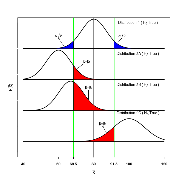
The Type I error for the specific example is depicted in the Distribution-1 of the Figure-1 below.
For a two sided null hypothesis which is actually true, the probability of observing a sample mean \(\small{\overline{x}}\) in the interval $(68.5, 91.5)$ around \(\small{\mu=80}\) is $95\%$. There is a $\alpha=0.05$ chance of observing \(\small{\overline{x}}\) value outside the inerval. This is the probability of making a Type I error.
We now consider the situation where
the alternate hypothesis is actually true. Let the distribution followed by the statistic under the true alternate hypothesis be as depicted in Distribution-2A in the Figure-1 above. Assume that the \(\small{\mu}\) value for this distribution
is not 80, but actually less than 80. We will never come to know this distribution. We will be only testing the null hypothesis following Distribution-1.
Since the alternate hypothesis is true, all the mean values \(\small{\overline{x}}\) on the Distribution-2 should be rejected by the test. However, because we are looking at the acceptance region $(68.5, 91.5)$ around \(\small{\mu=80}\) in the first curve, we will erroneously recognise the values of \(\small{\overline{x}}\) from Distribution-2 that lie in the region $(68.5, 91.5)$ to be accepting the null, while they are actually rejecting it!. This area $\beta=\beta_1$ is marked red in Distribution-2.
This fraction $\beta$ of statistic values that
fail to reject the null $H_0$ even though it is not true represent a type II error.
We test a null hypothesis to a significance level of \(\small{\alpha}\). If the null hypothesis $H_0$ is true, we are committing a Type I by rejecting $H_0$ in a fraction \(\small{\alpha}\) of tests when $H_0$ is actually true in all of them. Thus, the value $\alpha$ is the probability of comitting a type I error. This is fixed prior to the test when we choose $\alpha$.
On the other hand, if the alternate hypothesis $H_A$ is true, we commit a type II error by failing to reject the null $H_0$ in a fraction $\beta$ of tests when in reality alternate hypothesis $H_A$ is true in all the cases. The fraction $\beta$ is the probability of committing a Type II error.
The value of $\alpha$ is fixed by us, but $\beta$ can take many values .
In Figure-1 above, the Distrbution-2A, Distribution-2B and Distribution-2C represent type II errors $\beta$ for various alternate hypothesis corresponding to the null hypothesis shown in Distribution-1. We can see that this is not fixed, and can take many values depending on the distribution under alternate hypothesis.
Thus, in a classical hypothesis test of null ($H_0$) against the alternate ($H_A$), there are four possible decisions on outcomes,
two of which are right and remaining two are wrong:
- Accept the null $H_0$ when null is true (correct)
- Reject the null $H_0$ when null is false (correct)
- Reject the null $H_0$ when null is true ( Type-I error )
- Accept the null $H_0$ when null is false ( Type-II error)
The power of statistical test
The type II error \(\small{\beta}\) is the probability of failing to reject a false null hypothesis.
Therefore, the
quantity \(\small{1-\beta}\) is the probability that we will reject the false null hypothesis. \(\small{1-\beta}\) is called the power of statistical test .
We summarize the type I error, type II error and power as follows. It is easy to remember them with reference to null hypothesis being true or false:
1. If null hypothesis is true, we should accept it. If we fail to accept $H_0$ when it is true, we are committing a type I error with a probability \(\small{\alpha}\).
2. If the null hypothesis is false, we should reject it. If we fail to reject $H_0$ when it is false, we are committing a type II error with a probability \(\small{\beta}\).
3. If the null hypothesis is false, we should reject it. The probability of correctly rejecting $H_0$ is given by the power of statistical test \(\small{1-\beta}\).
In any statistical test, the significance level \(\small{\alpha}\) for rejecting the null hypothesis for the observed test statistic is fixed prior to the test. Therefore, the probability of committing a type I error is fixed. On the other hand, there are many test statistic values for accepting the alternate hypothesis. Therefore, the probabilty \(\small{\beta}\) of committing a type II error is not fixed, and it ca take many many values, depending on the parameters of the distribution followed by the alternate hypothesis.
The type I error \(\small{\alpha}\) and the type II error \(\small{\beta}\) are defined such that if one of them increases, the other decreases and vice versa. In Figure-1, note that as the blue area under Distribution-1 is increased by (movig the green vertical lines
), the red areas under distributions Distribution-2A, Distribution-2B and Distribution-2C.
The above fact implies that
if we try to reduce the type I error, the power of statistical test (ie., the ability to correctly reject the null hypothesis) is also decreased .
For a chosen value of \(\small{\alpha}\) to reject the null, We will never know the value of \(\small{\beta}\) since it dependes on the unknown distributions followed by the test statistic under alternate hypothesis. For a fixed value of \(\small{\alpha}\) and sample size n, the values of \(\small{\beta}\) and hence the power of test \(\small{\beta}\) can be computed for various assumed values of statistic when the alternate hypothesis is true. Such a plot is called
power curve. We will compute such curves for specific examples below.
Computing power functions for a statistical test
We will learn to compute the power function for a given hypothesis testing with specific examples, both for two sided and
one sided tests.
Example-1 : Compute power function for \(\small{~~~H_0 :~\mu~=~6,~~~~~~H_A :~\mu \neq 6,~~~~~~n=100,~~~~\sigma=1.4,~~~~~\alpha=0.05 }\)
Under null hypothesis, the sample mean \(\small{\overline{x}}\) follows a Gaussian \(\small{N(\mu, \dfrac{\sigma}{\sqrt{n}})}\)
For a two sided test with \(\small{\alpha=0,05}\), We first compute the $95\%$ interval around \(\small{\mu=6}\).
$95\%$ interval = \(\small{\mu \pm Z_{1-\alpha/2} \dfrac{\sigma}{\sqrt{n}}~=~6 \pm 1.96 \dfrac{1.4}{\sqrt{100}}~=~(5.72, 6.27 ) }\)
Under alternate hypothesis, we assume that \(\small{\overline{x}}\) is drawn from \(\small{N(\mu_A, \dfrac{\sigma}{\sqrt{n}})}\).
The probability of type II error \(\small{\beta}\) is the area under the curve \(\small{N(\mu_A, \dfrac{\sigma}{\sqrt{n}})}\) in the $95\%$ interval (5.72, 6.27) of the distribution \(\small{N(\mu_A, \dfrac{\sigma}{\sqrt{n}})}\) under Null hypothesis.
For the lower and upper bounds (5.72, 6.27) of sample mean, we compute Z statistics to get area under curve.
We compute,
\(\small{Z_1 = \dfrac{5.72 - \mu_A} {\dfrac{\sigma}{\sqrt{n}} } ~=~ \dfrac{5.72 - \mu_A} {\dfrac{1.4}{\sqrt{100}} }}\)
\(\small{Z_2 = \dfrac{6.27 - \mu_A} {\dfrac{\sigma}{\sqrt{n}} } ~=~ \dfrac{6.27 - \mu_A} {\dfrac{1.4}{\sqrt{100}} }}\)
Using the pnorm() function of R, we get \(~~~\small{\beta~=~P(Z_2) - P(Z_1)~=~pnorm(Z_2) - pnorm(Z_1) }\)
Thus, for various values of \(\small{\mu_A }\), we can compute \(\small{\beta}\) and hence the power of test \(\small{1-\beta}\) and plot the power curve between \(\small{\mu_A }\) and power.
The results are tabulated below:
| $\mu_A$ |
$\beta$ |
$1-\beta$ |
| $5$ |
$1.09 \times 10^{-7}$ |
$0.999$ |
| $5.2$ |
$8.69 \times 10^{-5}$ |
$0.999$ |
| $5.4$ |
$0.01$ |
$0.990$ |
$5.6$ |
$0.185$ |
$0.815$ |
$5.8$ |
$0.702$ |
$0.298$ |
$6.0$ |
$0.95$ |
$0.05$ |
$6.2$ |
$0.702$ |
$0.298$ |
$6.4$ |
$0.185$ |
$0.815$ |
$6.6$ |
$0.010$ |
$0.990$ |
$6.8$ |
$8.69 \times 10^{-5}$ |
$0.999$ |
$7.0$ |
$1.09 \times 10^{-7}$ |
$0.999$ |
The plot between $\mu_A$ values and the corresponding power $1-\beta$ is plotted in the Figure-2 below:
Example-2 : Compute power function for \(\small{~~~H_0~=~30,~~~~~~,H_A~\leq 30,~~~~~~n=100,~~~~\sigma=100,~~~~~\alpha=0.05 }\)
Since this is a left tailed test, we will fail to reject the null (and hence commit a type II error) if we get a
Z statistic greater than $-Z_{1-\alpha}~=~-Z_{0.95}~=~-1.645$.
The $95\%$ interval = \(\small{( \mu - Z_{1-\alpha} \dfrac{\sigma}{\sqrt{n}}, ~\infty) ~=~(30~-~ 1.645 \dfrac{100}{\sqrt{100}},~\infty)~=~(13.55, \infty ) }\)
Under alternate hypothesis, we assume that \(\small{\overline{x}}\) is drawn from \(\small{N(\mu_A, \dfrac{\sigma}{\sqrt{n}})}\).
The probability of type II error \(\small{\beta}\) is the area under the curve \(\small{N(\mu_A, \dfrac{\sigma}{\sqrt{n}})}\) in the $95\%$ interval (13.55, \infty) of the distribution \(\small{N(\mu_A, \dfrac{\sigma}{\sqrt{n}})}\) under Null hypothesis.
For the lower and upper bounds (13.55, \infty) of sample mean, we compute Z statistics to get area under curve.
We compute,
\(\small{Z_1 = \dfrac{13.55 - \mu_A} {\dfrac{\sigma}{\sqrt{n}} } ~=~ \dfrac{13.55 - \mu_A} {\dfrac{100}{\sqrt{100}} }}\)
\(\small{Z_2 = \infty }\)
Using the pnorm() function of R, we get \(~~~\small{\beta~=~P(Z_2) - P(Z_1)~=~pnorm(Z_2) - pnorm(Z_1) }\)
Thus, for various values of \(\small{\mu_A }\), we can compute \(\small{\beta}\) and hence the power of test \(\small{1-\beta}\) and plot the power curve between \(\small{\mu_A }\) and power.
The results are tabulated below: