CountBio

Suppose we make \(\small{n}\) repeated observations of some quantity represented by a variable name \(\small{x}\). Let us assume that these \(\small{n}\) observations denoted by \(\small{x_1,x_2,x_3,...,x_n}\) to have been randomly drawn('sampled') from a (parent) population of size N.

From the randomly drawn \(\small{n}\) samples, we can compute a statistic. The mean value \(\small{\overline{x}}\) of these n samples is computed using the standard formula,
\(~~~~~~~~~~\small{\overline{x} =\displaystyle{\sum_{i=1}^n}x_i =\dfrac{x_1 + x_2 + x_3 + .....+ x_n}{n} }\)

We assume \(\small{N \gg n }\) so that the random draw can be considered to be with replacement. Now we will draw another \(\small{n}\) samples from the population and compute their mean. This new mean \(\small{\overline{x}}\) will be different from the one we calculated for previous \(\small{n}\) samples. We repeat this by drawing all possible sets of n random samples that can be drawn from population of size N .

How many possible sample sets of size \(\small{n}\) can be drawn from a discrete population of size \(\small{N}\) with replacement?. It is actually \(\small{N^n}\) data sets, from which we compute \(\small{N^n}\) values of \(\small{\overline{x}}\).

Even if we draw \(\small{n=8}\) samples from a discrete population of size \(\small{N=100}\), we will end up with \(\small{100^8}\) possible sample data sets!. In the case of continuous distribution with infinite possible values, this task of getting all possible sample data sets is very very difficult task. If we have to do this practically, we can make an approximation by replacing "all possible sample data sets of size n" with "sufficiently large number of sample data sets of size n"

Assume that somehow we drew all possible sample data sets of size \(\small{n}\) from a population of size \(\small{N}\) and computed the sample mean \(\small{\overline{x}}\) for each one of them. We thus got a large number of mean \(\small{\overline{x}}\) values for sample size \(\small{n}\).

Suppose we plot a frequency distribution of these \(\small{\overline{x}}\) values. How will it look like?. Whats will be the mean and standard deviation of the distribution of this \(\small{\overline{x}}\) distribution?

First we give a name. The distribution \(\small{\overline{x}}\) is called the sampling distribution of mean for this population. Suppose we had computed median instead of mean, its distribution would be called "the sample distribution of median" for this parent population.

For a given population, the distribution of all possible values of a statistic computed from samples of finite size \(\small{n}\) drawn randomly with replacement from the population is called the sampling distribution of that statistic.

The distribution of sample mean

First we will find out the mean and standard deviation of the distribution of \(\small{\overline{x}}\) computed from \(\small{n}\) random samples.

Since computation of an \(\small{\overline{x}}\) involves the sum of \(\small{n}\) random samples from the population, the mean of many such \(\small{\overline{x}}\) values will involve summing up more and more data points from the distribution. So, in a large limit of \(\small{n}\), the mean of \(\small{\overline{x}}\) should approach the population mean \(\small{\mu}\).
We write this as,\(~~~~~~{\mu_{\overline{x}} = \mu}\)

Now we will derive an expression for the variance of the sample mean as follows:

Take the sum \(\small{\displaystyle{\sum_{i=1}^n}x_i}\) in the expression of \(\small{\overline{x}}\). This sum contains n random variables \(\small{x_i}\). Each one of them is identically distributed with a standard deviation \(\small{\sigma}\) of the population.

Therefore, we write

Variance(\(\small{\displaystyle{\sum_{i=1}^n}x_i) = \displaystyle{\sum_{i=1}^n}Variance(x_i) = \displaystyle{\sum_{i=1}^n}\sigma^2 = n\sigma^2 } \)

Next, we write down the variance of \(\small{\overline{x}}\).

Using the known result that for a constant k and a variable X, \(\small{Variance(kX) = k^2\times variance(X)}\), we write

\(\small{Variance(\overline{x}) = Variance(\dfrac{1}{n} \displaystyle{\sum_{i=1}^n}x_i) = \dfrac{1}{n^2} Variance(\displaystyle{\sum_{i=1}^n}x_i) = \dfrac{\sigma^2}{n} }\)

Thus we get this remarkable result :

If we randomly draw \(\small{n}\) samples from a distribution of a variable \(\small{x}\) with population mean \(\small{\mu}\) and variance \(\small{\sigma^2}\), then the computed mean \(\small{\overline{x}}\) of these samples follow a distribution whose mean and variance are given by,

\( ~~~~~~~~~~~~~~~\mu_{\overline{x}} = \mu ~~~~~~~~~~~~~~~~~ \)
\( ~~~~~~~~~~~~~~~\sigma_{\overline{x}}^2 = \dfrac{\sigma^2}{n}~~~~~~~~or~~~~\sigma_{\overline{x}} = \dfrac{\sigma}{\sqrt{n}} \)

This implies that the standard deviation of the sample mean \(\small{\overline{x}}\) is reduced by a factor equal to \(\small{\dfrac{1}{\sqrt{n}}}\), the inverse of the square root of the number of data points.

Since the standard deviation represents the error in the measurement about the mean value, the error on the computed \(\small{\overline{x}}\) can be reduced by incresing the number of data points!

The quantity \(~~~\dfrac{\sigma}{\sqrt{n}} \) is called the Standard Error of the Mean (SEM).

The correction due to finite sample size

In the above discussion we assumed that the population has a sample size \(\small{N}\) which is very very large when compared to the sample size \(\small{n}\). This is equivalent to sampling with replacement. However, if the population has a finite size \(\small{N}\) which is not very large compared to the sample size \(\small{n}\), and we draw without replacement, we need to apply a correction to the expression on \( \sigma_{\overline{x}} \).

For a population size \(\small{N}\) and a sample size \(\small{n}\), the expression for standard deviation on sample mean is written as,
\(~~~~~~~~~~~~~~~~~~~~~ \small{\sigma_{\overline{x}} = \dfrac{N-n}{N-1} \dfrac{\sigma}{\sqrt{n}} } ~~~~~~~~~~~~~~~\)

The value of the correction factor \(\small{\dfrac{N-n}{N-1}}\) approaches 1 as \(\small{N}\) gets larger and larger compared to \(\small{n}\). Approximately, if the population size is 20 times or more than the sample size, we can ignore this correction factor and use the usual expression \( \small{\sigma_{\overline{x}} = \dfrac{\sigma}{\sqrt{n}} } \)

The sampling distribution of a normal variable

If the population distribution of a random variable follows a normal distribution with mean \(\small{\mu}\) and standard deviation \(\sigma\), then it can be mathematically shown that the distribution of sample mean \(\small{\overline{x}}\) computed from \(\small{n}\) random samples of X is also Gaussian with mean \(\small{\mu}\) and standard deviation \(\small{\dfrac{\sigma}{\sqrt{n}}}\).

This can be verified by simulating random deviates from a normal distribution in R. We first generated 100000 random points (deviates) from a Gaussian with \(\small{\mu=30, \sigma=6 }\). The histogram of these points are plotted in the upper figure below. Because of the finite number of data points, the mean and standard deviation are 29.99 and 5.99, very close to 30 and 6 respectively. We then randomly sample 9 events from this Gaussian and estimate their mean \(\small{\overline{x}} \). We repeat this sampling 100000 times, and get the mean value for each data set. We then plot the histogram of these sample mean values, as shown in the lower figure below.

Freqeucy distribution of X and mean(X) from a Gaussian distribution

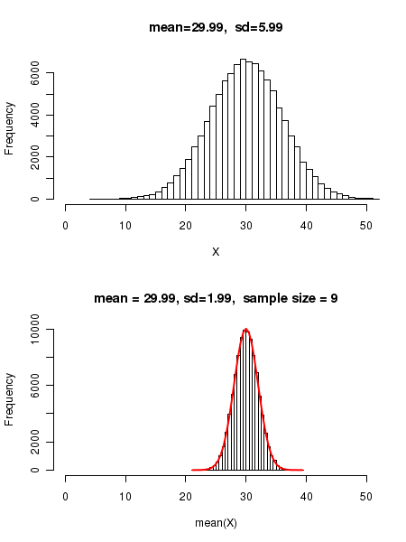
We notice in the lower figure that the standard deviation of mean is 2.99, which is very close to \(\small{\sigma_{\overline{x}} = \dfrac{\sigma}{\sqrt{n}}=\dfrac{6}{\sqrt{9}} = 3 }\), as expected. The red line in the lower plot is the density distribution of a Gaussian with \(\small{\mu=29.99}\) and \(\small{\sigma=1.99}\) normalized to 100000 data points. We can see that the Gaussian fits perfectly to the data histogram.

The effect of sample size on a measurement

When a quantity x is measured in an experiment, repeated measurements of under identical conditions are made and the mean is computed. Why should this be done?

Let us say, a variable \(\small{\overline{x}}\) has a population that follows a Gaussian distribution with mean \(\small{\mu}\) and a standard deviation \(\small{\sigma}\).

Suppose we make only a single observation in \(\small{\overline{x}}\). Since this observation is randomly chosen from the Gaussian with \(\small{N(\mu,\sigma)}\) , there is a high chance that the reading could be far away from the mean value. For example, in a Gaussian, there is \(\small{ 67\% }\) chance that a single observation is within one standard deviation around the mean and \(\small{ 33\% }\) chance it is more than a standard deviation away from mean \(\small{\mu}\).

On the other hand, let us repeat the measurement 36 times under identical conditions and compute the mean value \(\small{\overline{x}}\). Now the standard deviation (error) on this computed \(\small{\overline{x}}\) is not the same \(\small{\sigma}\), but reduced to \(\small{\dfrac{\sigma}{\sqrt{36}} = \dfrac{\sigma}{6}}\). The uncertanity on the computed mean is \(\small{\sqrt{n} }\) times less than the uncertainity on a single measurement.

If this is so, then what prevents us from repeating any experiment sufficiently large number of times (large n) to determine the mean very accurately?. Well, every measurement cost us resources like materials, money and time. Because of the square root factor on n in the expression, in order to reduce the error on mean by 10 times, we have to increase the observations 100 times!. This costs a lot!.