CountBio

After collecting the data, we have to summarize the data set to quantitatively describe it. Insted of presenting all the sample data points as a data set, one looks for a single number that can charactarizes the entire data set.

Such a number used for summarizing the whole data set is computed using the values of data points and is called a descriptive measure . There are many descriptive measures exist in statistical analysis.

The descriptive measures can be computed for the sample as well as population data.

A descriptive measure of the sample data is called a statistic .
A descriptive measure computed from the population data is called a parameter.

The descriptive measures can be broadly classified into the :following categories:

(1) The quantities that measure the central tendency in the data. They locate a particular value in the data space that can be taken as a data summary with certain properties. The important descriptive measures that measure the central tendency are:

• Mean (arthmetic, geometric and harmonic means)
• Median

• Range
• Variance
• Standard deviation

• Mode
• Percentiles and quartiles

• Skewness
• Kurtosis

Arithmetic Mean

The arithmetic mean is the most important measure of central tendency, and is widely used throught the statistical analysis.

To understand the mean, let us consider data points labelled as \( x_1, x_2, x_3, .... \) from the repeated measurements of a variable \( x \). We just plot them as points along an axis such that their distance from an origin point O represents their value. See figure below:

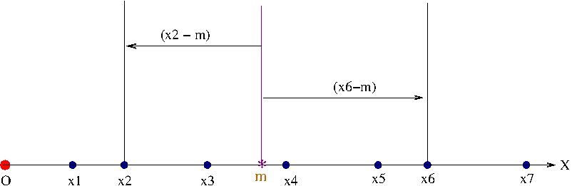
Suppose, we want a value 'm' to be the best representation of the "central tendency" of the data set X. What criterian we should use to compute such a number?.

One way of going about this is as follows: We can think of m as a number around which all the data points are somewhat "optimally" positioned. For such an optimization, we have to choose a measure.

One such measure can be the deviation of data points from the central tendency.

We can find the deviation of each data point from \( m \) and sum it. But the differences can be positive as well as negative, and hence may cancel each other in the sum. To avoid this, we sqaure the difference of each data point from \( m \) and sum. We thus declare a sum S as,

\(~~~~~~~~~~~~~~S = (x_1 - m)^2 + (x_2 - m)^2 + ....+ (x_n - m)^2 = \sum\limits_{i=1}^{n} (x_i - m)^2 \)

There are infinite number of choices for the location of m between first and last point. For every value we choose for m, there will be a corresponding sum value S. The most optimal value of m is the one that minimizes the sum S.

This is achived by minimizing the expression for S with respect to m. We thus differentiate S with respect to m, equate to zero and get an expression for m in terms of \(x_i \). (For minima, second derivative should also go to zero). Thus we write,

\(\dfrac{dS}{dm} = \dfrac{d}{dm}\sum\limits_{i=1}^{n} (x_i - m)^2 = 0 \)
\(\sum\limits_{i=1}^{n} (x_i - m) = 0 \)
\(\sum\limits_{i=1}^{n} x_i - \sum\limits_{i=1}^{n}m = \sum\limits_{i=1}^{n} x_i - mn = 0 \)
\( m = \dfrac{1}{n} \sum\limits_{i=1}^{n} x_i \)

Also, the second derivative of S with respect to m given by \(\dfrac{d^2}{dm^2} \sum\limits_{i=1}^{n} (x_i - m)^2 \) is positive.

Therefore, the expression \( m = \dfrac{1}{n} \sum\limits_{i=1}^{n} x_i \) as a measure of central tendency minimizes the sum square deviation of data points from its value. This quantity is called the arithmetic mean of the data set. This is also called the average value of the data. This expression is same for the sample data as well as the population. In the case of population, n is the size of the entire population .

In literature, it is customary to use the greek letter \( \mu \) ('mu') for the population mean and an 'overbar' on any variable to represent its sample mean (eg., sample mean of variable X is \( \overline{X}\).

Thus the expression for arithmatic mean is,

The arithmetic mean is one of the most important statistical parameters. It is so important that the word "mean" refers to the arithmetic mean. However, there are two more mean values are used as central measures. We will learn them now.

The law of large numbers

According to the law of large numbers , the arithmetic mean from the sample converges to the expected mean \( \small{\mu}\) of the population as the sample size increases. ie.,

\(~~~~~~~~\overline{x} \rightarrow \mu~~~as~~~n \rightarrow \infty\)

Geometric Mean

The geometric mean of n numbers \( x_1, x_2, x_3, ...., x_n \) is the \( n^{th} \) root of their product. Thus,

Note that, by virtue of its definition, the geometric mean goes to zero if any one of the numbers is zero.

The geometric mean is used as a central measure of a data set which represents the fractional (percentage) growth, where the data points are related to each other. On the other hand, the arithmetic mean is a good central measure of data points which are independent of each other . We will understand this with an example.

The number of offsprings born to cows in a diary farm during three successive years is given as 122, 148 and 171 respectively. Since these numbers represent absolute changes which are not related to each other, we can compute the mean number of offsprings born over the three years using arithmetic mean:

\( \small{~~~~~~~~~~~~~~~~~Mean~number~of~offsprings = \dfrac{122+148+171}{3} = 147 }\)

Suppose another diary farm gives the yearly data on the cattle growth as the percentage increase in population when compared to the previous year . Starting with N cattle in the beginning, first year had an increase of 1.2 times the beginning, the second year it was 1.9 times the first year, and during third year the growth in the number was 2.3 times the second year.

Let m be the central measure of fractional increase that replaces these 3 numbers. Then, on the third year, we should have,

\( \small{~~~~~~~~~~~~~~~~N \times 1.2 \times 1.9 \times 2.3 = N \times m \times m \times m } \)
This gives a geometric mean of growth rate as, \( \small{~~~~m = (1.2 \times 1.9 \times 2.3)^{\dfrac{1}{3} } } = 1.737\) per year.

We will now find the arithmetic mean of growth rate:

\(\small{~~~~~~~~~~~~~~~~m = \dfrac{1.2+1.9+2.3}{3} = 1.8 }\)

We will compare our results.

Using geometric mean of growth rate, fractional increase after 3 years = \( (1.737)^3 = 5.240. \), close to the actual product \( 1.2 \times 1.9 \times 2.3 = 5.243 \).

Using arthmetic mean of growth rate, fractional increase after 3 years = \( (1.8)^3 = 5.832 \).

We see that in this case, the geometric mean is a better central measure. The geometric mean is appropriate in the situations where effects are multiplicative, wheras arithmetic mean is useful when the effects are additive.

Taking exponential on both sides, we get the geometric mean of a,b,c,d.

The above property is very useful in finding the geometric mean of very large number of data points.

Thus, if {\( x_1, x_2, x_3, ....., x_n \)} are n data points with large values, their product becomes huge. We can take a mean of their logarithmic values and exponentiate it to get their geometric mean.

Harmonic mean

The harmonic mean of n numbers \(x_1,x_2,x_3,....,x_n \) is given by,

From this expression we describe a harmonic mean as the reciprocal of the arithmetic mean of the reciprocals .

The harmonic mean is used when we have to find the average of rates of quantities and fractions. For example, if we want to find the average of three velocities given as \( \small{ 32 Km/s, 45 Km/s} \) and \(\small{52 Km/s }\), we can compute their harmonic mean, which will give better result than the arithmetic mean.

Median

For a finite data set, the median is the value of the variable such that half of the data points have values more than the median and half of the data points have values less than the median.

To find the median of a data set, following procedure is adopted:

When we have large outliers in the data points, median is a better central measure compared to mean. The mean value is more sensitive to large outliers than the median. The following two examples illustrate this:

We notice that when compared to median, the value of mean is more sensitive to outliers.

When to use the Arithmetic mean, Harmonic mean, Geometric mean and the Median?

We will summarize the uses of the three means and the median for a sample data set X:

Arithmetic mean \( {\small = \overline{X} = \dfrac{1}{n} \sum\limits_{i=1}^{n} x_i~~~~~~~~~}\) (When the data points are simple numbers).

Geometric mean = \( \small{X_{GM} = (x_1 \times x_2 \times x_3 \times .... \times x_n )^{\dfrac{1}{n}}}~~~~~~~~~ \) (When data are fractions or percentages )

Harmonic mean = \( \small{ m_H = \dfrac{n}{\sum\limits_{i=1}^n \dfrac{1}{x_i}} }~~~~~~~~~~ \)(When the data points are rates )

Median = middle value \(~~~~~~~~~~\) (for simple numbers with outliers).

Variance and the Standard deviation

The variance is a measure of deviation of the data points from their mean. This is an important parameter in describing any statistical distribution.

Consider n observations \( { x_1, x_2, x_3,....,x_n } \) of a variable which are supposed to have drawn randomly from a population. We determine the sample mean of this data to be \( \overline{x} = \dfrac{1}{n} \sum\limits_{i=1}^{n} x_i \).

Let \( \mu \) be the mean of the population from which data points are drawn.

The deviation \((x_i - \mu) \) of a data point from the population mean is called statistical error .

The deviation \((x_i - \overline{x}) \) of a data point from the sample mean is called residual error.

The variance of a population is the the mean square deviation of the data points from the population mean :

The variance of a sample data is the the mean square deviation of the data points from the sample mean:

Notice the important difference in the two formulas. The variance of the population has \(n \) dividing the sum wheras the variance of the sample has \( n-1 \) dividing the sum. We will explain this important difference in detail since we will encounter this in the definition of many parameters:

Reason for dividing by (n-1) for the computation of sample variance

The data points of the sample are assumed to have been randomly drawn from a population. Any statistic we estimate from the n data points using a formula will not be exactly equal to the corresponding parameter value of the population. However, suppose we repeat the exepriment very very large number of times, by drawing n random data points from population everytime and estimate the statistic using a formula. The mean (expectation) value of these large(infinite number of) repeats will then exactly be equal to the parameter of the population. If that happens, then that statistic is called the unbiased estimator of the parameter.

For a given parameter of the population, there is a particular formula using which we compute the corresponding statistic from data points that will make the statistic the unbiased estimator of that parameter. This formula is derived from a mathematical method called maximum likelihood estimates . We will not describe this method here, but will take the results from this method.

Using this method it can be shown that, if \( {\small \mu = \dfrac{1}{n}\sum\limits_{i=1}^{n}x_i }\) is the expression for computing mean for a population, then \( {\small \overline{X} = \dfrac{1}{n}\sum\limits_{i=1}^{n}x_i }\) computed from sample data gives the unbiased estimate of \( \mu \).

Using the same method, it can be shown that if \( {\small \sigma^2 = \dfrac{1}{n}\sum\limits_{i=1}^{n}(x_i - \overline{x})^2 }\) is the expression for computing variance from population, then \( {\small s^2 = \dfrac{1}{n-1}\sum\limits_{i=1}^{n}(x_i - \overline{x})^2 }\) computed from the sample data is the unbiased estimate of \( \sigma^2 \). The (n-1) instead of n in the denominator (mathematically) comes from the requirement that the variance \( s^2 \) computed from the data should be an unbiased estimate of \( \sigma^2 \) of the population.

Another way of understanding (n-1) is through the concept of degrees of freedom . The number of independent parameters required to compute a quantity is called degrees of freedom. For example, the calculation of the mean requires all the n data points, and hence has n degrees of freedom .

In the case of sample data, it can be shown that the sum \(\sum\limits_{i=1}^{n}(x_i - \overline{x}) = 0 \)

From the above relation, if we have (n-1) data points and their mean value, we can determine the \( n^{th} \) data point. Thus, the computation of the variance has only (n-1) independent data points and hence has (n-1) degrees of freedom . Because of this, the sum of deviations is divided by (n-1) to compute the average.

Since the variance is a square of the difference, we define a quantity called standard deviation as the square root of the variance . The standard deviations of the population and the sample are accordingly defined using their variance as,

The standard deviation is a direct measure of error in the data, as we will learn in the later lessons.

Mode

The mode of a data set is the value that occurs maximum number of times.

In the data set \( \small{\{5,3,7,5,8,9,12,5,2,9,5,7,5\} }\), the number 5 repeats maximum number (four) of times, when compared to other values. Hence the mode of this data set is 5.

If more than one value occur maximum number of times, each one of them can be considered as a mode, and the data is said to be multimodal .

Thus in the data set \( \small{\{22,34,86,56,22,11,22,34,78,68,34 \} }\), the numbers 22 and 34 both occur maximum number of times, which is three. This data is bimodel.

If data points are drawn from a continuous distribition , there may not be any repeat numbers. In this case, we should construct a frequency histogram. The data interval corresponding to the highest bin height in the histogram should be treated as the mode.

In the case of a continuous probability distribution described by a formula, the variable value corresponding to the peak should be taken as mode. If the distributio is symmetric (like Gaussian) then the mean, median and mode may be same.

If a continuous distribution has multiple peaks, then each peak should be called a mode which make this distribution multimodel .

Percentiles and Quartiles

Order statistics and Rank of a data : If we take a data set X consisting of n observations and arrange them in ascending order , the resulting ordered data are called the order statistics of the data sample.

As an illustration, consider the following data consisting of 60 measurements from an experiment:

                            Data set X :

        44 69 53 57 54 57 71 67 53 55 79 52 71 69 61

        62 53 69 52 70 49 55 45 51 66 46 66 66 44 53 

        65 66 58 63 59 52 78 60 53 71 58 67 65 73 79

        35 46 66 67 42 59 63 50 52 50 51 71 56 38 69
       

We now arrange the above data X in ascending order to create an ordered data which we name as Y, as shown below:

               Ordered data set Y  :

       35 38 42 44 44 45 46 46 49 50 50 51 51 52 52 

       52 52 53 53 53 53 53 54 55 55 56 57 57 58 58 

       59 59 60 61 62 63 63 65 65 66 66 66 66 66 67 

       67 67 69 69 69 69 70 71 71 71 71 73 78 79 79

For the above ordered data set Y, we give a rank to each element and use it as a subscript.
Thus, first element \( \small{y_i = 35} \) is called the first order statistic and has rank 1.
The fourth element \( \small {y_i = 44} \) is called the fourth order statistic and has rank 4.

Since the elements are ordered, we have \( \small{y_1 \lt y_2 \lt y_3 \lt .....\lt y_{60} } \)

From the order statistics, we define a Pth sample percentile as the data point which has P% of the data points below it and (100-P)% of data points above it.

According to this definition, the median is the 50th sample percentile, since 50% of data points are less than the median and 50% of the data points are above it.

For an order statistics Y, we can find the \(P^{th}\) percentile point using the following method:

If n is the number of data points, compute the value \(~~~~~ \small{ m = (n+1)\dfrac{P}{100} } \)

If m turns out be an integer, then \( \pi_P = y_m\) is the Pth percentile point.

If m is not an intger but a fraction, write is as sum of an integer r and a fraction f. For example, if m=34.6, r=34 and f=0.6.

Then the Pth sample percentile is given by, \(~~~~~~ \pi_P = y_r + f(y_{r+1} - y_r) \)

In the above step, we have found a weighted average of \(r^{th} \) and \( (r+1)^{th} \) statistics.

Among the percentile points, the following three are very important:

The 25th percentile point is called the First quartile

The 50th percentile point is called the second quartile , which is also the median of the data.

The 75th percentile point is called the third quartile .

The difference between third and the first quartile is called interquartile distance

Box and Whisker plot for the data description

A box and whisker plot is made up of a box at the center with three quartiles marked on it. From the end of the box, two whiskers are extended along both sides to touch the maximum and minimum points in the data. The outliers are also marked as points above and below the whiskers, if needed.

Suppose, for a given data set we compute the parameters as follows:

         min = 4.4,  Q1=5.2, median=5.4, Q3=5.6, max=6.1 

where min and max are minimum and maximum points of the data set, Q1 is first quartile and Q3 is third quartile. The Box and whisker plot for this data is shown here:

Box and Whisker Plot

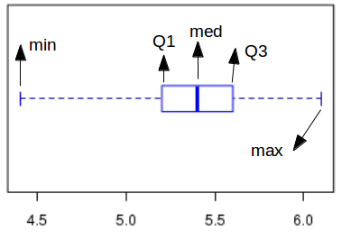
Outliers in the data : When the data has supposed to have outliers (extreme points), the whiskers are extended upto points excluding these outlier points. For an arbitrary number 'm', the data points with values m*(Q3-Q1) above Q3 or m*(Q3-Q1) below Q1 are declared as outliers, and are represented by circles beyong the whiskers.

Skewness

R scripts

R statistical package has many built in functions to compute the statistical parameters. We will describe some of them and demonstrate their usage in an R script.

 x  ---------->  A data vector of numbers.

 min(x, na.rm=FALSE) -------> Returns the minimum value of the data. 
                                 If  na.rm=FALSE, will return NA if the data contains one or more NA (default).
                                 na.rm=TRUE will ignore th NA values to return the minimum.

 max(x, na.rm=FALSE) -------> Returns the maximum value of the data. 
                                 If na.rm=FALSE, will return NA if the data has one or more NA (default).
                                 na.rm=TRUE will ignore th NA values to return the maximum.

 mean(x, na.rm=FALSE) -------> Returns the arithmetic mean of the data vector x.
                                 If na.rm=FALSE, will return NA if the data has one or more NA (default).
                                 na.rm=TRUE will ignore th NA values to return the mean value.

 var(x, na.rm=FALSE) -------> Returns the variance of the data vector x.
                                 If na.rm=FALSE, will return NA if the data has one or more NA (default).
                                 na.rm=TRUE will ignore th:w NA values to return the variance.



 sd(x, na.rm=FALSE) -------> Returns the standard deviation of the data vector x.
                                 If na.rm=FALSE, will return NA if the data has one or more NA (default).
                                 na.rm=TRUE will ignore th NA values to return the standard deviation.

quantile(x,probs,type=6,na.rm=TRUE) --------> Returns the percentile point of the ordered data of x.
                                 Will work only if na.rm=TRUE. Will not work with NA's
                                 probs -- a vector or list of percentile values(in fraction) between 0-1.
                                 For example, probs=0.5 returns median, probs=0.6 computes 60th percentile.
                                 type--> decides the algorithm for computing the percentile.
                                 type=6 uses the algorithm described in this lesson.


 summary(x)  --------> Returns the statistical summary of data vector x as list with 7 elements.
                         Generic function that can be used to summarize the outputs of many more functions.
                         The returned list contains minimum, first quartile, median, mean, third quartile,
                         maximum and the number of NA's in the data.

The R script shown here demonstrates the computation basic statistical parameters using R library functions:

## Computing statistical parameters in R

## Define a data vector
 x = c(51.4,36.3,45.9,49.5,46.9,48.5,50.0,45.0,44.2,46.0,41.9,42.4,50.7,41.4,41.2)

## Find the minimum value
 xmin = min(x) 
 print(paste("minimum = ", xmin))

## Find the maximum value
 xmax = max(x)
 print(paste("minimum = ", xmax))
 
## Compute the arithmetic mean
 armean = mean(x)
 print(paste("arithmetic mean = ", armean))

## Compute the geometric mean.
## Here, we compute log( [x1*x2*...*xn]^(1/n) ) and take its exponential.
## If numbers are large, direct products will become unmanagable. Hence this method.
 geomean =  exp((1/length(y)) * sum(log(y)))
 print(paste("geometric mean = ", geomean))

## Compute the harmonic mean
 harmean = length(y)/sum(1/y) 
 print(paste("harmonic mean = ", harmean))

## Compute the median function
 med = median(x)
 print(paste("median = ", med))

## compute the 0,25,50,75 and 100th percentile points:
 yq = quantile(x, type=6)
 print("0, 25, 50, 75 and 100 percentile points :  ")
 print(yq)

## Get the interquartile range from the above data
 IQrange = yq[4]-yq[2]
 print(paste("The interquartile range (Q3-Q1) = ", IQrange))

## Get the 37th percentile point
 per37 = quantile(x, probs=0.37, type=6)
 print(paste("The 37th percentile = ", per37))

## Get the 20th and 80th percentile points
 per2080 = quantile(x, probs=c(0.2,0.8), type=6)
 print(paste("The 20th and 80th percentile points = ", per2080[1], "   ", per2080[2]))

## Compute a data summary using summary() function
 datsum = summary(x)
 print("Data summary with summary() function : ")
 print(datsum)

Running the above script generates the output as shown here:

[1] "minimum =  36.3"
[1] "maximum =  51.4"
[1] "arithmetic mean =  45.42"
[1] "geometric mean =  44.6581090931252"
[1] "harmonic mean =  44.3033340683336"
[1] "median =  45.9"
[1] "0, 25, 50, 75 and 100 percentile points :  "
  0%  25%  50%  75% 100% 
36.3 41.9 45.9 49.5 51.4 
[1] "The interquartile range (Q3-Q1) =  7.6"
[1] "The 37th percentile =  44.056"
[1] "The 20th and 80th percentile points =  41.5     49.9"
[1] "Data summary with summary() function : "
   Min. 1st Qu.  Median    Mean 3rd Qu.    Max. 
  36.30   42.15   45.90   45.42   49.00   51.40