CountBio

Non-parametric tests for unpaired samples

These tests are non-parametric equivalent of two sample independent t-test.

We will describe two such tests which are closely related:

1. Wilcoxon rank sum test for unpaired samples

2. Mann-Whitney U test for two unpaired samples

These tests are based purely on the order in which observations from the two samples fall. They test is used for two comparing two continuous variables that may not follow Gussian distribution.

They test the null hypothesis that the two data samples X and Y come from the same population against an alternative that observations in one sample tend to be larger than the observations in the other.

The basic assumptions for the tests are:

(i) The two distributions X and Y are continuous and need not be Gaussian.

(ii) The observations are ordinal.

(iii) The two distributions X and Y have the same shape. Any difference between them is due to the shift in one distribution with respect to the other, which changes only their median, and not the shape. See the figure below:

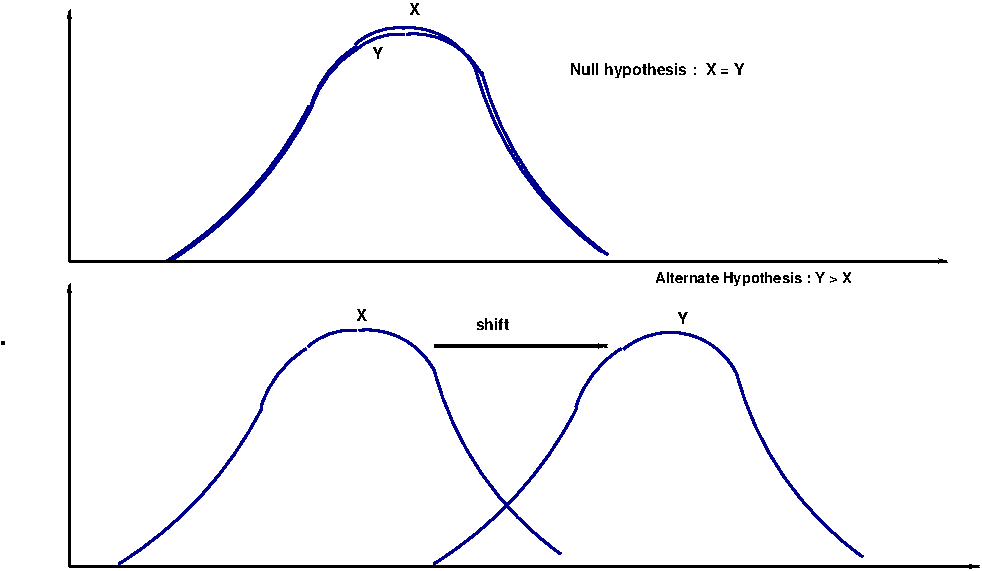
Thus these tests detect the shift in the two distributions under the assumptions that their shapes are same.

Because of this, we can construct the null hypothesis for testing two distributions X and Y in many ways like

"Null hypothesis that \(\small{X=Y}\) against an alternatives \(\small{X \gt Y }\), \(\small{X \lt Y }\) and \(\small{X \neq Y }\)"

"Null hypothesis that median of X equals median of Y against alternative hypothesis on their inequalities"

These two tests are testing essentially the same thing. Also, the expression for their statistic differ just by an additive constant involving sample sizes. Because of this, "Wilcoxon rank sum test" is also called as "Wilcoxon-Mann-Whitney test". Similarly, "Mann-Whitney U test" is also called as "Mann-Whitney-Wilcoxon test". In this section, we describe both the test one below other.

1. Wilcoxon rank sum test for unpaired samples

Let \(\small{x_1,x_2,x_3,....,x_{n_1} }~\) and \(\small{y_1,y_2,y_3,.....,y_{n_2}~}\) be the samples of sizes \(\small{n_1}\) and \(\small{n_2}\) drawn randomly from two continuous distributions X and Y respectively. Let \(\small{m_X}\) and \(\small{m_Y}\) be the respective medians of the populations X and Y.

In the Wilcoxon signed rank test, we test the null hypothesis \(\small{~H_0:m_X \gt m_Y}\) against an alternate hypothesis \(\small{H_A:m_X \gt m_Y }~\) or \(~\small{H_A:~m_X \lt m_Y }\).

$~~~~~~~~~~~~~~~~~~~~~~~~~~~~~~~~~~~$ Procedure for computing test statistic

1. The two sets of observations are,

\(~~~~~~~~\small{X~=~\{x_1,x_2,x_3,....,x_{n_1}\} }~\)

\(~~~~~~~~\small{Y~=~\{y_1,y_2,y_3,....,y_{n_2}\} }~\)

2. Merge the two sets of data points into one single set of size \(\small{n=n_1+n_2}\) and rank them. Carefully tag each data point in the two sets with its rank in the combined set. (All the ranks are positive)

In the case of repeats, replace their individual ranks by theie mean ranks.

3. Now separate the two data sets remembering the of their individual data points in the combined set. Create a rank sum of the members for each data set separately. Let

\(\small{~~~~~~W_X~=~ }\) Sum of ranks for observations from X

\(\small{~~~~~~W_Y~=~ }\) Sum of ranks for observations from Y

4. Take \(\small{W~=~min(W_X,W_Y)}\) to be the Wilcoxon test statistic. (This decision is arbitrary. We can also take \(\small{max(W_X,W_Y)}\) to be the test statistic.)

$~~~~~~~~~~~~~~~~~~~~~~~~~~~~~~~~~~~~~~~~~~~~~~$ Hypothesis testing

If the distribution Y has shifted to the right with respect to the distribution X (as in Figure-1 above), the values of data set Y will tend to be larger than the values of X as compared to the case when the two distributions are same. In this case, \(\small{W=W_x }\). The null hypothesis \(\small{H_0:m_X = m_Y }\) will tend to be defeated against an alternate \(\small{H_A:m_X \lt m_Y }\) for smaller and smaller values of \(\small{W=W_x }\). Therefore, the critical region for testing \(\small{H_0:m_X = m_Y }\) against an alternate \(\small{H_A:m_X \lt m_Y }\) will be of the form \(\small{W \leq W_c }\).

Similarly, if the distribution Y has shifted to the left with respect to the distribution X, the values of data set X will tend to be larger than the values of Y as compared to the case when the two distributions are same. In this case, \(\small{W=W_Y }\). The critical region for testing \(\small{H_0:m_X = m_Y }\) against an alternate \(\small{H_A:m_Y \lt m_X }\) will be of the form \(\small{W \leq W_c }\).

For a two sided test with \(\small{H_0: m_X = m_Y}\) against an alternative \(\small{H_0: m_X \neq m_Y }\), reject null if \(\small{W \leq W_{lower}~ }\) or \(\small{W \geq W_{upper}~}\), using a lower or upper critical value.

In order to compute the critical values like wc, we need the probability distribution W. This can be computed by two methods:


Method-1 : Direct computation :

We combine \(\small{n_1}\) data points from X and \(\small{n_2}\) data points from Y and rank the \(\small{n=n_1+n_2}\) data points. We thus get ranks \(\small{R_i}\), where \(\small{i=1,2,3,....,n }\) for n data points. \(\small{n_1}\) of these ranks go to data set X and the remaining \(\small{n_2}\) go to data set y when we separate them.

Under the null hypothesis \(\small{H_0: m_x=m_Y }\), each rank \(\small{R_i}\) has equal probability of being assigned to the data set X or Y. We form all possible pairs of ranks (\(\small{R_i, R_j}\)) for (X,Y) and take their rank sums.

For example, let X has 2 data points and Y has 3 data points. The assigned ranks will be (1,2,3,4,5).

The possible combinations of rank pairs ( \(\small{R_i,R_j)}\) are,

(1,2),(1,3),(1,4),(1,5),(2,1),(2,3),(2,4),(2,5),(3,1),(3,2),(3,4),(3,5),

(4,1),(4,2),(4,3),(4,5),(5,1),(5,2),(5,3),(5,4)

Under null hypothesis, probability of observing (\(\small{R_i,R_j}\)) is same as the probability of observing (\(\small{R_i,R_j}\)), we are left with the following pairs and their rank sums:

$~~~~~~~~~~~~~~~~~~~~~~~~$ Rank Pairs $~~~~~~~~~~$Rank sums (W)
$~~~~~~~~~~~~~~~~~~~~~~~~$----------------$~~~~~~~~~~$-------------------
$~~~~~~~~~~~~~~~~~~~~~~~~~~~~~$(1,2)$~~~~~~~~~~~~~~~~~~~~~~~3~$
$~~~~~~~~~~~~~~~~~~~~~~~~~~~~~$(1,3)$~~~~~~~~~~~~~~~~~~~~~~~4~$
$~~~~~~~~~~~~~~~~~~~~~~~~~~~~~$(1,4)$~~~~~~~~~~~~~~~~~~~~~~~5~$
$~~~~~~~~~~~~~~~~~~~~~~~~~~~~~$(1,5)$~~~~~~~~~~~~~~~~~~~~~~~6~$
$~~~~~~~~~~~~~~~~~~~~~~~~~~~~~$(2,3)$~~~~~~~~~~~~~~~~~~~~~~~5~$
$~~~~~~~~~~~~~~~~~~~~~~~~~~~~~$(2,4)$~~~~~~~~~~~~~~~~~~~~~~~6~$
$~~~~~~~~~~~~~~~~~~~~~~~~~~~~~$(2,5)$~~~~~~~~~~~~~~~~~~~~~~~7~$
$~~~~~~~~~~~~~~~~~~~~~~~~~~~~~$(3,4)$~~~~~~~~~~~~~~~~~~~~~~~7~$
$~~~~~~~~~~~~~~~~~~~~~~~~~~~~~$(3,5)$~~~~~~~~~~~~~~~~~~~~~~~8~$
$~~~~~~~~~~~~~~~~~~~~~~~~~~~~~$(4,5)$~~~~~~~~~~~~~~~~~~~~~~~9~$

Since each one of these 10 pairs have equal probability 1/10, we get the probabilities of various rank sum values:

$~~~~~~~~~~~~~~~~~~~~~~~~$ Rank Sum (W) $~~~~~~~~~~$P(W)
$~~~~~~~~~~~~~~~~~~~~~~~~$----------------$~~~~~~~~~~$-------------------
$~~~~~~~~~~~~~~~~~~~~~~~~~~~~~$3$~~~~~~~~~~~~~~~~~~~~~~~$1/10
$~~~~~~~~~~~~~~~~~~~~~~~~~~~~~$4$~~~~~~~~~~~~~~~~~~~~~~~$1/10
$~~~~~~~~~~~~~~~~~~~~~~~~~~~~~$5$~~~~~~~~~~~~~~~~~~~~~~~$2/10
$~~~~~~~~~~~~~~~~~~~~~~~~~~~~~$6$~~~~~~~~~~~~~~~~~~~~~~~$2/10
$~~~~~~~~~~~~~~~~~~~~~~~~~~~~~$7$~~~~~~~~~~~~~~~~~~~~~~~$2/10
$~~~~~~~~~~~~~~~~~~~~~~~~~~~~~$8$~~~~~~~~~~~~~~~~~~~~~~~$1/10
$~~~~~~~~~~~~~~~~~~~~~~~~~~~~~$9$~~~~~~~~~~~~~~~~~~~~~~~$1/10

From this we can compute cumulative probabilities like,

\(\small{P(W \leq 5)~=~1/10~+~1/10~+~2/10~=~4/10 }\)

For various sample sizes \(\small{n_1}\) and \(\small{n_2}\),the rank sum values corresponding to cumulative probabilities \(\small{\alpha }\) are computed and tabulated. This Wilcoxon rank sum table for 2 samples can be used for hypothesis testing. See here for such a table.

Summary of decision rules for the critical value table:

Compute the rank sum values \(\small{W_X}\) and \(\small{W_Y}\) from data with \(\small{n_1}\) and \(\small{n_2}\) data points.

Take \(\small{W=min(W_X,W_Y)}\) to be the Wilcoxon test statistic.

From the Wilcoxon rank sum table, get the critical value \(\small{W_c}\) for a given \(\small{n_1,n_2}\) and \(\small{\alpha }\).

Reject \(\small{H_0:m_X = m_Y }\) against a one sided alternate \(\small{H_A:m_X \lt m_Y }\) if \(\small{W \geq W_c(n_1,n_2,\alpha) }\).

Reject \(\small{H_0:m_X = m_Y }\) against a one sided alternate \(\small{H_A:m_Y \lt m_X }\) if \(\small{W \leq W_c(n_1,n_2,\alpha) }\).

For a two sided test with \(\small{H_0: m_X = m_Y}\) against an alternative \(\small{H_0: m_X \neq m_Y }\), reject null if \(\small{W \leq W_{c}(n_1,n_2,\alpha/2)~~ }\) or \(~~\small{W \geq W_{c}(n_1,n_2,1-\alpha/2)~ }\)

Remember that \(\small{W_c(n_1,n_2,1-\alpha/2)~=~W_c(n_1,n_2,~n_1n_2-\alpha/2) }\)


Method-2 : Large sample approximation :

When the sample sizes are large (both \(\small{n_1}\) and \(\small{n_2}\) values are around 10), an approximation can be made to provide a distribution for the Wilcoxon statistics W.

When n is large, under the null hypothesis that both the distributions are X and Y equal, the distribution of W can be approximated to be a Gaussian whose mean and variance (for the choice of \(\small{W=W_Y}\) are given by,

\(\small{~~~~~~~~~~~~~~\mu_W~=~\dfrac{n_2(n_1+n_2+1)}{2}~~~~~~~~}\) and \(~~~~~\small{\sigma_W^2~=~\dfrac{n_1n_2(n_1+n2+1)}{12} }\)

Employing central limit theorem, we can write down a Z staistic for W under the null hypothesis \(\small{H_0}\) as,

\(\small{~~~~~~~~~Z~=~\dfrac{W-\dfrac{n_2(n_1+n_2+1)}{2}}{\sqrt{\dfrac{n_1n_2(n_1+n_2+1)}{12}}}~~~~}\)is N(0,1), approximately a unit normal distribution.

Once the Z statistics is computed from the data, we can get the corresponding p-values and critical regions for a significance level of \(\small{\alpha }\) from unit Normal distribution to test the null hypothesis against one or two sided alternate hypothesis.

Mann-Whitney U test for unpaired samples

Let x1,x2,x3,....,xn1 and y1,y2,y3,.....,yn2 be the samples of sizes \(\small{n_1}\) and \(\small{n_2}\) drawn randomly from two continuous distributions X and Y respectively. Let \(\small{m_x}\) and \(\small{m_Y}\) be their respective medians.

In Mann Whiteney test, every sample \(\small{x_i}\) in the data set X is compared with every other sample \(\small{y_j}\) in the second data set. Thus we have \(\small{n_1n_2}\) pairs of comparisons.

If the two samples have same median under a null hypothesis, then each \(\small{x_i}\) has equal probability of being greater or smaller than each \(\small{y_j}\) in a pair of comparison.ie.,

Under null hypothesis,\(~~\small{H_0:~P(x_i \gt y_j)~=~\frac{1}{2} }\)
Under alternate hypothesis, ,\(~~\small{H_A:~P(x_i \gt y_j)~\neq~\frac{1}{2} }\)

Among the \(\small{n1n2}\) possible pairs \(\small{(x_i,y_j) }\), count the number of times \(\small{x_i \gt y_j}\). Call this number \(\small{U_X }\). Similarly, count the number of times \(\small{y_j \gt X_i}\). Call this number \(\small{U_Y}\).

The minimum among \(\small{U_X}\) and \(\small{U_Y }\) is taken to be the Mann-Whitney U statistic. \(~~~~\small{U~=~min }\)

We then go to the statistical table for Mann-Whitney test to get the probability of observing this U value or lower. For a one sided test, this is the p-value. If the test is two sided, double this probability to obtain the p-value.

$~~~~~~~~~~~~~~~~~~~~~~~~~~~~~~~~~~~$ Procedure for computing test statistic

The method follwed is almost same as that of Wilcoxon test procedure described above. We firs compute Wilcoxon test statistic W and from that get Mann-Whitney test statistic U. We repeat this procedure here again for the sake of clarity:

1. The two sets of observations are,

\(~~~~~~~~\small{X~=~\{x_1,x_2,x_3,....,x_{n_1}\} }~\)

\(~~~~~~~~\small{Y~=~\{y_1,y_2,y_3,....,y_{n_2}\} }~\)

2. Merge the two sets of data points into one single set of size \(\small{n=n_1+n_2}\) and rank them. Carefully tag each data point in the two sets with its rank in the combined set. (All the ranks are positive)

In the case of repeats, replace their individual ranks by their mean.

3. Now separate the two data sets remembering the of their individual data points in the combined set. Create a rank sum of the members for each data set separately. Let

\(\small{~~~~~~W_X~=~ }\) Sum of ranks for observations from X

\(\small{~~~~~~W_Y~=~ }\) Sum of ranks for observations from Y

4. Two values \(\small{U_X}\) and \(\small{U_Y}\) are defined as,

\(\small{~~~~~~~~~~U_X~=~W_X~-~\dfrac{n_1(n_1+1)}{2} }\)

\(\small{~~~~~~~~~~U_Y~=~W_Y~-~\dfrac{n_2(n_2+1)}{2} }\)

4. Take \(\small{min(U_X,U_Y)}\) to be the Mann-Whitney U statistic. (This decision is arbitrary. We can also take \(\small{max(W_X,W_Y)}\) to be the test statistic.)



$~~~~~~~~~~~~~~~~~~~~~~~~~~~~~~~~~~~~~~~~~~~~~~$ Hypothesis testing

If the distribution Y has shifted to the right with respect to the distribution X (as in Figure-1 above), the values of data set Y will tend to be larger than the values of X as compared to the case when the two distributions are same. In this case, \(\small{U=U_x }\). The null hypothesis \(\small{H_0:U_X = U_Y }\) will tend to be defeated against an alternate \(\small{H_A:U_X \lt U_Y }\) for smaller and smaller values of \(\small{U=U_x }\). Therefore, the critical region for testing \(\small{H_0:m_X = m_Y }\) against an alternate \(\small{H_A:m_X \lt m_Y }\) will be of the form \(\small{U \leq U_c }\).

Similarly, if the distribution Y has shifted to the left with respect to the distribution X, the values of data set X will tend to be larger than the values of Y as compared to the case when the two distributions are same. In this case, \(\small{U=U_Y }\). The critical region for testing \(\small{H_0:m_X = m_Y }\) against an alternate \(\small{H_A:m_Y \lt m_X }\) will be of the form \(\small{U \leq U_c }\).

For a two sided test with \(\small{H_0: m_X = m_Y}\) against an alternative \(\small{H_0: m_X \neq m_Y }\), reject null if \(\small{U \leq W_{lower}~ }\) or \(\small{U \geq U_{upper}~}\), using a lower or upper critical value.

In order to compute the critical values like Uc, we need the probability distribution U. This can be computed by two methods:


Method-1 : Direct computation :

For various values of sample sizes n1,n2 and significance level \(\small{\alpha }\), critical values \(\small{U_c }\) have been computed and tabulated Mann-Whitney test tables. From this, we can read the critical values for staistical test.


Method-2 : Large sample approximation :

When the sample sizes are large (ie., \(\small{n_1}\) and \(\small{n_2}\) both are 10 are more), the distribution of U is approximated to be a Gaussian with \(\small{~~\mu_U~=~\dfrac{n_1n_2}{2}}~~\) and \(~~\small{\sigma_U^2~=~\dfrac{n_1n_2(n_1+n_2+1)}{12} }\).

Using Central Limit Theorem, we write a Z statistics that follows a unit normal distribution:

\(\small{~~Z~=~\dfrac{U~-~\dfrac{n_1n_2}{2}}{\sqrt{n_1n_2(n_1+n_2+1)}}~~\rightarrow~~N(0,1) }\)

Using the Z statistic computed for the data, we can perform a one sided or two sided hypothesis test.

R-scripts

The Wilcoxon family of tests can be performed in R using the wilcox.test() function.

Important functon parameters are:

wilcox.test(x, y = NULL, alternative = c("two.sided", "less", "greater"),
                 mu = 0, paired = FALSE, exact = NULL, correct = TRUE,
		 conf.int = FALSE, conf.level = 0.95, ...) 

 x, y  -------> two data vectors. y=NULL makes it a single vriable test.

 alternative  ------>  type of alterntive hypothesis. 

 mu  ------> population mean to be compare. zero by default

paired   -----> In the case of two sample test, are the samples paired or not?

exact  ------>  a logical indicating whether an exact p-value should be computed.
                                          By default, exact=NULL

 correct  ---- a logical indicating whether to apply continuity correction
          in the normal approximation for the p-value.

 conf.int  ---- a logical indicating whether confidence intervl should be computed.

 conf.level  ---- confidence level for the test.

## Wilcoxon rank sum test test for two independent  variables

## Note : If there are ties, exact confidence interval cannot be clculatedby this method.


## we test a null that the two distributions are equal with an alternative that placebo is smaller than the drug
##   (ie., pain due to drug has reduced with when compared to placebio)

drug = c(31.7,75.0,101.1,60.5,62.8,59.3,58.9,91.3,99.1,52.0,39.1)

placebo = c(59.3,72.7,100.5,64.7,69.0,72.7,69.6,97.4,100.6,65.1,65.7)

res = wilcox.test(drug,placebo, conf.level=0.95, alternative=c("greater"), conf.int=TRUE )

print(res)

Executing the above script in R prints the following output.

	Wilcoxon rank sum test with continuity correction

data:  drug and placebo
W = 38.5, p-value = 0.9303
alternative hypothesis: true location shift is greater than 0
95 percent confidence interval:
 -25.99998       Inf
sample estimates:
difference in location 
             -9.199981