Gauss-Newton method for nonlinear least square
minimization
The nonlinear least square method for estimating the coefficients $b_1, b_2, b_3,...,b_n$
involves the minimization of the residual sum function given by,
\begin{equation}
\displaystyle\sum_{i=1}^n e_i^2~=~
\displaystyle\sum_{i=1}^n [y_i~-~g(b_1,b_2,b_3,....,b_p;~~x_{i1},x_{i2},x_{i3},....,x_{im})]^2
\end{equation}
$~~~~~~~~~(1)$
where,
g() is the nonlinear function to be fitted with n data points $(x_i, y_i)$
$b_1,b_2,b_3,....,b_p~~$ are the p parameters of the model
$x_{i1},x_{i2},x_{i3},....,x_{im}~~$ are the m variables in the model
$\overline{b}=\{b_1,b_2,b_3,....,b_p\} ~~$ is a vector of coefficients
$\overline{x}_i=\{x_{i1},x_{i2},x_{i3},....,x_{im}\}~~$ is the vectors of parameters for
the data point i.
With the above definitions of various symbols, we write the sumsquare function as,
\begin{equation}
f(\overline{b})~=~
\dfrac{1}{2}\displaystyle\sum_{i=1}^n [y_i~-~g(\overline{b}, \overline{x}_i)]^2
\end{equation}
$~~~~~~~~~~~~(2)$
where we have included an arbitrary constant $\dfrac{1}{2}$ which will be cancelled when
we take the derivative of $f(\overline{b})$ with respect to the coefficients.
The residual for the $i^{th}$ data point is,
\begin{equation}
r_i(\overline{b})~=~
[y_i~-~g(\overline{b}, \overline{x}_i)]
\end{equation}
$~~~~~~~~~~(3)$
With this, we write the sumsquare function $f(\overline{b})$ as,
\begin{equation}
f(\overline{b})~=~
\dfrac{1}{2}\displaystyle\sum_{i=1}^n r_i^2
\end{equation}
$~~~~~~~~~~~~(4)$
We have to now minimize the above function f with respect to coefficients b.
The simplest way of doing this will be to use Newton's method. The Newton's method of
solving a system of n equations minimizes the function f:
In Newton's method of finding solutions to nonlinear equations
for a single variable B, the system of n equations to iterate is given by,
${B^{k+1} ~= B^k~-~\dfrac{f'(B^k)}{f''(B^k)} }~~~~~$ Here, k=1,2,3,4... is number of iteration.
The general form of above iteration equation can be written for a vector of p coefficients
$\overline{b}$ and m variables $\overline{x}$ as,
\begin{equation}
\overline{b}^{k+1}~= \overline{b}^{k}~-~ ( {\overline \nabla}^2 f(\overline{b}^{k}))^{-1}
{\overline \nabla} f(\overline{b}^{k})
\end{equation}
$~~~~~~~~~~(5)$
where $\overline{b}^k$ denotes the values of coefficients $b_1, b_2,b_3,...,b_p$ in the $k^{th}$
iteration of Newton's method.
The above equation (5) is a set of p iterative equations for p coefficients $b_1,b_2,...,b_p$.
For example, for the coefficient $b_3$, we write
\( b_3^{k+1}~= b_3^{k}~-~ ( {\overline \nabla}^2 f(\overline{b}^{k}))^{-1}
{\overline \nabla} f(\overline{b}^{k}) \)
One important problem encountered in using Newton's method is, the above iterative procedure
that uses first and second derivatives is not guaranteed to converge for the nonliear least
square procedure. The main reason for this is that the search direction may not be the descend direction
of the function f from the current point.
One way of solving this issue is to use th Gauss-Newton method for iterative minimization.
In this method, the first and second derivatives in the iterative procedure of equation (5) are written
in terms of Jacobian of the function f with respect to vairiables b. In this modified Newton's procedure,
the search direction is guaranteed to be the discend direction.
Derivation of Gauss-Newton algorithm
We should get the first and second derivatives if residual sum function f with respect to
the coefficients b.
Differentiating equation(4) with respect to b,
\begin{equation}
\dfrac{\partial f}{\partial b_j}~=~
\displaystyle \sum_{i=1}^n \dfrac{\partial r_i}{\partial b_j} r_i~=~
\displaystyle \dfrac{\partial r_1}{\partial b_j} r_1~+~
\displaystyle \dfrac{\partial r_2}{\partial b_j} r_2~+~
\displaystyle \dfrac{\partial r_3}{\partial b_j} r_3~+~
.......... +~
\displaystyle \dfrac{\partial r_n}{\partial b_j} r_n
\end{equation}
$~~~~~~~~~~(6)$
where the index j=1,2,3,...,p corresponds to parameters of the model.
The gradient of the function $f(\overline{b})$ is,
\[
\overline \nabla f~=~
\begin{bmatrix}
\displaystyle \dfrac{\partial f}{\partial b_1} \\
\displaystyle \dfrac{\partial f}{\partial b_2} \\
\displaystyle \dfrac{\partial f}{\partial b_3} \\
..... \\
..... \\
\displaystyle \dfrac{\partial f}{\partial b_p}
\end{bmatrix}
~=~
\begin{bmatrix}
\displaystyle \dfrac{\partial r_1}{\partial b_1} r_1~+~&
\displaystyle \dfrac{\partial r_2}{\partial b_1} r_2~+~&
\displaystyle \dfrac{\partial r_3}{\partial b_1} r_3~+~&
........~+~&
\displaystyle \dfrac{\partial r_n}{\partial b_1} r_n \\
\displaystyle \dfrac{\partial r_1}{\partial b_2} r_1~+~&
\displaystyle \dfrac{\partial r_2}{\partial b_2} r_2~+~&
\displaystyle \dfrac{\partial r_3}{\partial b_2} r_3~+~&
........~+~&
\displaystyle \dfrac{\partial r_n}{\partial b_2} r_n \\
\displaystyle \dfrac{\partial r_1}{\partial b_3} r_1~+~&
\displaystyle \dfrac{\partial r_2}{\partial b_3} r_2~+~&
\displaystyle \dfrac{\partial r_3}{\partial b_3} r_3~+~&
........~+~&
\displaystyle \dfrac{\partial r_n}{\partial b_3} r_n \\
..... &.....&.....&.....&......\\
..... &.....&.....&.....&......\\
\displaystyle \dfrac{\partial r_1}{\partial b_p} r_1~+~&
\displaystyle \dfrac{\partial r_2}{\partial b_p} r_2~+~&
\displaystyle \dfrac{\partial r_3}{\partial b_p} r_3~+~&
........~+~&
\displaystyle \dfrac{\partial r_n}{\partial b_p} r_n \\
\end{bmatrix}
\]
The above gradian matrix can be written as the multiplication of the following two matrices:
\[
\overline \nabla f~=~
\begin{bmatrix}
\displaystyle \dfrac{\partial r_1}{\partial b_1} &
\displaystyle \dfrac{\partial r_1}{\partial b_2} &
\displaystyle \dfrac{\partial r_1}{\partial b_3} &
...... &
\displaystyle \dfrac{\partial r_1}{\partial b_p} \\
\displaystyle \dfrac{\partial r_2}{\partial b_1} &
\displaystyle \dfrac{\partial r_2}{\partial b_2} &
\displaystyle \dfrac{\partial r_2}{\partial b_3} &
...... &
\displaystyle \dfrac{\partial r_2}{\partial b_p} \\
\displaystyle \dfrac{\partial r_3}{\partial b_1} &
\displaystyle \dfrac{\partial r_3}{\partial b_2} &
\displaystyle \dfrac{\partial r_3}{\partial b_3} &
...... &
\displaystyle \dfrac{\partial r_3}{\partial b_p} \\
... & ...& ... & ......& ... \\
... & ...& ... & ......& ... \\
\displaystyle \dfrac{\partial r_n}{\partial b_1} &
\displaystyle \dfrac{\partial r_n}{\partial b_2} &
\displaystyle \dfrac{\partial r_n}{\partial b_3} &
...... &
\displaystyle \dfrac{\partial r_n}{\partial b_p} \\
\end{bmatrix}
^{\huge T}
\begin{bmatrix}
r_1 \\
\\
r_2 \\
\\
r_3 \\
\\
... \\
\\
... \\
\\
r_n
\end{bmatrix}
\]
We identify the Jacobian Mareix of vector $\overline r$ to be
\[
\overline{J}_r~=~
\begin{bmatrix}
\displaystyle \dfrac{\partial r_1}{\partial b_1} &
\displaystyle \dfrac{\partial r_1}{\partial b_2} &
\displaystyle \dfrac{\partial r_1}{\partial b_3} &
...... &
\displaystyle \dfrac{\partial r_1}{\partial b_p} \\
\displaystyle \dfrac{\partial r_2}{\partial b_1} &
\displaystyle \dfrac{\partial r_2}{\partial b_2} &
\displaystyle \dfrac{\partial r_2}{\partial b_3} &
...... &
\displaystyle \dfrac{\partial r_2}{\partial b_p} \\
\displaystyle \dfrac{\partial r_3}{\partial b_1} &
\displaystyle \dfrac{\partial r_3}{\partial b_2} &
\displaystyle \dfrac{\partial r_3}{\partial b_3} &
...... &
\displaystyle \dfrac{\partial r_3}{\partial b_p} \\
... & ...& ... & ......& ... \\
... & ...& ... & ......& ... \\
\displaystyle \dfrac{\partial r_n}{\partial b_1} &
\displaystyle \dfrac{\partial r_n}{\partial b_2} &
\displaystyle \dfrac{\partial r_n}{\partial b_3} &
...... &
\displaystyle \dfrac{\partial r_n}{\partial b_p} \\
\end{bmatrix}
\]
We thus finally get an expression for the gradiant of r in terms of its Jacobian matrix:
\( \overline \nabla f ~=~ {\overline{J_r}}^T {\overline r} \)
$~~~~~~~~~~(7)$
Now we derive an expression for the second derivative of the sumsquare function f.
Taking the derivative of equation (6) with respect to b gives the second derivative of f with respect
to the parameters b:
\begin{equation}
\dfrac{\partial^2 f}{\partial b_j \partial b_k}~=~
\displaystyle {\sum_{i=1}^{n} \left( \dfrac{\partial r_i}{\partial b_j}
\dfrac{\partial r_i}{\partial b_k} + r_i \dfrac{\partial^2 r_i}{\partial b_i \partial b_k} \right)}
\end{equation}
$~~~~~~~~(8)$
Using equation(8), we write the Hessian of second derivative matrix for the function f as,
\begin{equation}
{\overline H}_f~=~ \overline{\nabla}^2 f ~=~{\overline J}_r^T {\overline J}_r~+~\displaystyle
\sum_{i=1}^n r_i \overline{\nabla}^2r
\end{equation}
$~~~~~~~~~~~~~~(9)$
The equation(9) is the matrix version of equation(8) for all the parameters $b_1, b_2,...,b_p$
of the model.
In the Gauss-Newton method, the term $\displaystyle \sum_{i=1}^n r_i \overline{\nabla}^2
r $
is neglected from the expression for second derivative :
Neglecting this term, we write the Hessian (secon derivative) matrix as,
\begin{equation}
\overline{H}_f~=~ \overline{\nabla}^2 f~=~{\overline J}_r^T {\overline J}_r
\end{equation}
$~~~~~~~~~(10)$
Equation(7) and equation(10) give the first and second derivative of function f respectively
in terms of the Jacobian matrix of r. We can use the first and second derivative in Newton's method
to get the coefficients b through iterative procedure.
For a function with single variable x, we have seen that the iterative procedure for Newton's
method is written as,
${B^{k+1} ~= B^k~-~\dfrac{f'(B^k)}{f''(B^k)} }$
In our problem with p parameters of the model, the Gauss-Newtom iteration prcedure is
written interms of jacobian matrices of r as,
\begin{equation}
{\overline b}^{k+1}~=~{\overline b}^{k}~-~
\left[ \displaystyle \left[\overline{J}_r(\overline{b}^k)\right]^{T}
\overline{J}_r(\overline{b}^k) \right]^{-1}
\displaystyle \left[\overline{J}_r(\overline{b}^k)\right]^{T} \overline{r}(\overline{b}^k)
\end{equation}
$~~~~~~~~~~~~~~(11)$
The advantage of Gauss-Newton method
1. The second derivative need not be computed.
The Jacobinas with first derivative is used for solving the iterative procedure to estimate
the coefficients b.
2. The search direction is always the descent direction
so long as the jacobian matrix ${\overline J}_r(\overline{x}^k)$ has full rank.
In Newton's method, because of the use of first and second derivatives, the search direction
is not guaranteed to be the descending direction from an initial value of the parameter.
Example Calculation for Gauss-Newton method
In this section, we will fit a nonlinear function using Gauss-Newton method.
For this we choose a data set between an independent variable X and a dependent variable Y.
We fit a nonlinear function which represents the Michaelis-Menton formula of enzyme kinetics.
The function is of the form,
$ y~=~\dfrac{b_1 x}{b_2+x}~~~~~$ where $b_1$ and $b_2$ are the coefficients of the model.
The data set is given below:
\[
\begin{array}{|c|c|}
\hline
\text{x} & \text{y} \\
\hline
1.0 & 24.52 \\
1.5 & 30.81 \\
2.0 & 32.65 \\
2.5 & 34.45 \\
3.0 & 38.58 \\
3.5 & 38.22 \\
4.0 & 37.08 \\
4.5 & 38.64 \\
5.0 & 40.76 \\
5.5 & 43.51 \\
7.0 & 42.64 \\
9.0 & 46.01 \\
10.0 & 46.60 \\
12.0 & 47.53 \\
14.0 & 46.24 \\
16.0 & 47.32 \\
18.0 & 45.78 \\
20.0 & 48.15 \\
\hline
\end{array}
\]
The residual for data point i is given by,
$r_i~=~y_i - \dfrac{b_1 x_i}{b_2 + x_i} $
The partial derivatives of the residual with respect to the two parameterx $b_1$ and $b_2$
for each data point i are given by,
$ \dfrac{\partial r_i}{\partial b_1}~=~\dfrac{-x_i}{b_2 + x_i}~~~~~~~~~~~~~~~$(A)
$\dfrac{\partial r_i}{\partial b_2}~=~\dfrac{b_1 x_i}{(b_2 + x_i)^2}~~~~~~~~~~~$(B)
For a given value of $b_1$ and $b_2$, the Jacobian matrix is computed using
equations (A) and (B)given above for the 18 data points:
\[
\overline{J}_r~=~
\begin{bmatrix}
\dfrac{\partial r_1}{\partial b_1} & \dfrac{\partial r_1}{\partial b_2} \\
\dfrac{\partial r_2}{\partial b_1} & \dfrac{\partial r_2}{\partial b_2} \\
\dfrac{\partial r_3}{\partial b_1} & \dfrac{\partial r_3}{\partial b_2} \\
....... & ....... \\
....... & ....... \\
\dfrac{\partial r_{18}}{\partial b_1} & \dfrac{\partial r_{18}}{\partial b_2} \\
\end{bmatrix}
\]
With this information, we set up an iterative procedure to compute the eofficients $b_1$
and $b_2$. The steps of the iteration are as follows:
STEP-1:
Let us start with a set of initial values : $~~b_1=35~~$, $b_2~=~2$.
For these $b_1$ and $b_2$ values, compute and tabulate the following quantities:
\[
\begin{array}{|c|c|}
\hline
\text i &\text{x_i} & \text{y_i} & \dfrac{\partial r_i}{\partial b_1}~=~\dfrac{-x_i}{2 + x_i}
& \dfrac{\partial r_i}{\partial b_2}~=~\dfrac{35 x_i}{(2 + x_i)^2} & r_i~=~y_i - \dfrac{b_1 x_i}{b_2 + x_i}\\
\hline
1& 1.0& 24.5222& -0.3333& 3.8889& 12.8555 \\
2& 1.5& 30.8157& -0.4286& 4.2857& 15.8157 \\
3& 2.0& 32.6491& -0.5000& 4.3750& 15.1491 \\
4& 2.5& 34.4460& -0.5556& 4.3210& 15.0016 \\
5& 3.0& 38.5818& -0.6000& 4.2000& 17.5818 \\
6& 3.5& 38.2228& -0.6364& 4.0496& 15.9501 \\
7& 4.0& 37.0849& -0.6667& 3.8889& 13.7516 \\
8& 4.5& 38.6397& -0.6923& 3.7278& 14.4089 \\
9& 5.0& 40.7648& -0.7143& 3.5714& 15.7648 \\
10& 5.5& 43.5118& -0.7333& 3.4222& 17.8451 \\
11& 7.0& 42.6428& -0.7778& 3.0247& 15.4206 \\
12& 9.0& 46.0069& -0.8182& 2.6033& 17.3705 \\
13& 10.0& 46.6046& -0.8333& 2.4306& 17.4379 \\
14& 12.0& 47.5339& -0.8571& 2.1429& 17.5339 \\
15& 14.0& 46.2385& -0.8750& 1.9141& 15.6135 \\
16& 16.0& 47.3244& -0.8889& 1.7284& 16.2133 \\
17& 18.0& 45.7811& -0.9000& 1.5750& 14.2811 \\
18& 20.0& 48.1509& -0.9091& 1.4463& 16.3327 \\
\hline
\end{array}
\]
The Jacobian matrix and the r matrix for this first iteration i=1 are written as,
\[
\overline{J}_r(\overline{b}^1)~=~
\begin{bmatrix}
-0.3333 & 3.8889 \\
-0.4286 & 4.2857 \\
-0.5000 & 4.3750 \\
-0.5556 & 4.3210 \\
-0.6000 & 4.2000 \\
-0.6364 & 4.0496 \\
-0.6667 & 3.8889 \\
-0.6923 & 3.7278 \\
-0.7143 & 3.5714 \\
-0.7333 & 3.4222 \\
-0.7778 & 3.0247 \\
-0.8182 & 2.6033 \\
-0.8333 & 2.4306 \\
-0.8571 & 2.1429 \\
-0.8750 & 1.9141 \\
-0.8889 & 1.7284 \\
-0.9000 & 1.5750 \\
-0.9091 & 1.4463 \\
\end{bmatrix}
~~~~~~~~~~~\overline{r}({\overline b}^1)~=~
\begin{bmatrix}
12.8555 \\
15.8157 \\
15.1491 \\
15.0016 \\
17.5818 \\
15.9501 \\
13.7516 \\
14.4089 \\
15.7648 \\
17.8451 \\
15.4206 \\
17.3705 \\
17.4379 \\
17.5339 \\
15.6135 \\
16.2133 \\
14.2811 \\
16.3327 \\
\end{bmatrix}
\]
STEP-2:
Once the Jacobian and R matrices are computed, we compte the mareix product as,
\[
\left[ \displaystyle \left[\overline{J}_r(\overline{b}^1)\right]^{T}
\overline{J}_r(\overline{b}^1) \right]^{-1}
\displaystyle \left[\overline{J}_r(\overline{b}^1)\right]^{T} \overline{r}(\overline{b}^1)
~=~
\begin{bmatrix}
-14.2271 \\
1.8143 \\
\end{bmatrix}
\]
STEP-3:
Once the jacobian product is there, we iterate using equation(11) to get the second iteration
values of $b_1$ and $b_2$ as,
\begin{equation}
{b_1}^{2}~=~{b_1}^{1}~-~(-14.2271)~=~35+14.2271~=~49.2271
\end{equation}
\begin{equation}
{b_2}^{2}~=~{b_1}^{1}~-~(1.8143)~=~2 - 1.8143~=0.1857
\end{equation}
Now Go back to Step-1 with $b_1={b_1}^{2}~~~~~$ and $~~~~b_2 ={b_2}^{2}$ and proceed to get
third iteration
values ${b_1}^{3}~$ and $~{b_2}^{3}$ and so on until the different between two successive
iteration values fall below a pre-set threshold number
For example, the first ten iterations in R package yielded the following values
for $b_1% and $b_2$:
[1] "b1 =  49.2270821479973     b2= 0.18567571269335"
[1] "b1 =  48.3525681412689     b2= 0.703162497047043"
[1] "b1 =  49.8862567438057     b2= 1.01047436901084"
[1] "b1 =  50.1455775188186     b2= 1.05946832057398"
[1] "b1 =  50.1561575807817     b2= 1.06117954696531"
[1] "b1 =  50.1563926667571     b2= 1.06121189470479"
[1] "b1 =  50.1563970246927     b2= 1.06121248954209"
[1] "solution values converged within 1e-5 after  7  iterations"
[1] "b1 =  50.1563970246927     b2= 1.06121248954209"
For an arbitrary error threshold of $1.0\times 10^{-5}$, we got a convergence within 7
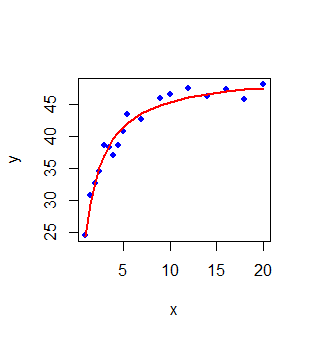
iterations, giving a value of $b_1 = 50.15639$ and $b_2 = 1.061212$ as final estimates.
The plot of fitted values $y_{fitted} = \dfrac{50.156~ x}{1.0612 + x}$ versus the observed values
is shown in the plot of Figure-1 below. In this plot, the blue points represent the data and
the red line is the regression line of Michaelis-Menton relationship:
Nonlinear Regression with R - basic script
The R-script below follows the theoretical steps of Gauss-Newton algorithms discussed in the
prvious example section.

It performs nonlinesr regression for the same Michaelis-Menton data we discussed.

The data from table-1 is stored in the simple text file  MM_kinetics_data.csv and the script below reads it into a data frame:
## This is the basic script implementing Gauss Newton minimization of
##   nonlinear functions.

## nonlinear function form :  y = b1*x/(b2+x)

##  ri = yi - (b1*xi)(b2+xi)  ## residual of data point i

##  d/db1(ri) = -xi/(b2+xi)  ## partial derivative of residual ri w.r.to b1

##  d/db2(ri) = b1*xi/(b2+xi)^2 ## partial derivative of residual ri w.r.to b2


## read the data file from MM kinetics

dat = read.csv(file="MM_kinetics_data.csv", header=TRUE)

##plot(dat$x, dat$y)


##

xdat = dat$x
ydat = dat$y

#Start with some initial value for the two parameters
b1 = 35
b2 = 2.0

## loop for iterative estimate of parameters

for(i in 1:30){

  ## residual matrix
  r = ydat - ((b1*xdat)/(b2+xdat))

  rmatrix = as.matrix(r)

  ## Partial derivatives of residual r with respect to coefficients b1 and b2
  partial_b1 = -xdat/(b2+xdat)

  partial_b2 = b1*xdat/(b2+xdat)^2

## Compute the jacobian matrix for current parameter vaoues
  dj = data.frame(partial_b1, partial_b2)

  Jmatrix = as.matrix(dj)

## product of jacobian matrix and residual matrix
  Jprod = solve(t(Jmatrix) %*% Jmatrix) %*% t(Jmatrix) %*% rmatrix

## Store parameter values for current iteration
  b1_before = b1
  b2_before = b2

## update parameter values
  b1 = b1 - Jprod[1,1]
  b2 = b2 - Jprod[2,1]

## store updated parameter values
  b1_after = b1
  b2_after = b2

## print the previous and updated parameter values
  print(paste("b1 = ", b1_after, "    b2=", b2_after))

## If-condition for breaking the iteration.
## When the differene between current b parameters and previous iteration values is less than 1e-5,
## break the loop
## The number 1e-5 is arbitrary. Can be chosen to be smaller for more accurate estimats of b parameter values.

  if( ( abs(b1_after - b1_before) <  1e-5 ) && ( abs(b2_after - b2_before) <  1e-5 )){

     print(paste("solution values converged within 1e-5 after ", i, " iterations"))

     print(paste("b1 = ", b1_after, "    b2=", b2_after))

  break
  }

}

##  Plot the data points and the fitted curve

y_fitted = b1*xdat/(b2 + xdat)

plot(xdat, ydat, col = "blue", pch = 18)
lines(xdat, y_fitted, col="red", type="l", lwd=2)

##--------------------------------------------------------------------
Running the above script in R prints the following output lines and graph on the screen:
[1] "b1 =  49.2270821479973     b2= 0.18567571269335"
[1] "b1 =  48.3525681412689     b2= 0.703162497047043"
[1] "b1 =  49.8862567438057     b2= 1.01047436901084"
[1] "b1 =  50.1455775188186     b2= 1.05946832057398"
[1] "b1 =  50.1561575807817     b2= 1.06117954696531"
[1] "b1 =  50.1563926667571     b2= 1.06121189470479"
[1] "b1 =  50.1563970246927     b2= 1.06121248954209"
[1] "solution values converged within 1e-5 after  7  iterations"
[1] "b1 =  50.1563970246927     b2= 1.06121248954209"
Nonlinear Regression with R library functions
In R, the function nls() performs the linear regression of data between two vectors.
 It has the option

for weighted and non-weighted fits, as well as nonlinear curve fitting.

The function call with essential parameters is of the form,

 nls(formula, data, start, weights)

where,

 formula  ------>  is the formula used for the fit. For linear function, use "y~x"

 data  -------->  data frame with x and y columns for data

 start  ------> a list consisting of initial values of parameters

 weights  ------> an optionl vector with weights of fits to be used.
The default method of nonlinear regression in nls() is Gauss-Newton method.
Consult the manual of R stats libary for other methods available.
For many additional parameters and their usage, type
help(nls) in R.
The R script below shows how to perform linear regression .
## Fitting MM kinetics (nonlinear) curve using nls function.

## read the table into a data frame
dat = read.csv(file="MM_kinetics_data.csv", header=TRUE)

# rename the data columns
y = dat$y
x = dat$x

## call the nls function with data, formula and initial values for the parameters
res <- nls(y ~ (b1 * x) / (b2 + x), start=list(b1=35, b2=2.0))

## print the summary of results
print(summary(nls))

## Plot the data ponts and fitted line
plot(x,y,col="blue", pch=20, cex=1.3)
lines(x, predict(res), type="l", lwd=2, col="red")
Running the above script in R prints the following output lines and graph on the screen:
Formula: y ~ (b1 * x)/(b2 + x)

Parameters:
   Estimate Std. Error t value Pr(>|t|)
b1 50.15639    0.66250   75.71  < 2e-16 ***
b2  1.06121    0.07473   14.20 1.73e-10 ***
---
Signif. codes:  0 ‘***’ 0.001 ‘**’ 0.01 ‘*’ 0.05 ‘.’ 0.1 ‘ ’ 1

Residual standard error: 1.294 on 16 degrees of freedom

Number of iterations to convergence: 6
Achieved convergence tolerance: 1.971e-06