CountBio

Analysis of Gene Expression Data
from microarrays

A microarray experiment results in a set of image files, one file per sample, obtained from the scanner. The conversion of the image intensities to gene expression data involves many complicated steps of analysis. These steps and the methodologies followed vary between different technologies used.

However, a common thread runs between these methods. In this section, we will describe the important steps involved in the construction of gene expression from the probe level intensity measurement made by the scanner.

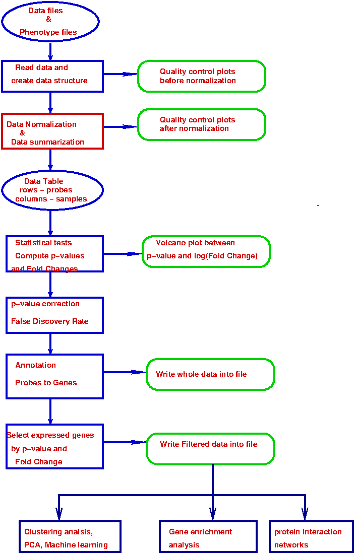
Figure-1 below is a block diagram of various steps involved in a microarray data analysis in general. We will describe these steps one by one while pointing out how these steps are implemented in the analysis of data from affymetrix genchip technology. We have prioritised the Affymetrix technology due to its dominance in terms of reliability and predominance in gene expression measurments across various conditions when compared to other methods like Illumina and Agilent two dye methodologies. We may include these analysis in this web page in future.


Now we will describe these steps upto the estimation of the differential gene expression. Other downstreame analysis methods like gene enrichment analysis, clustering and Principal component analysis will be described elsewhere.

Step-1 : Getting the Data and phenotype files

The first step in the microarray data analysis is to collect the basic data files from the scanner along with their supporting files and keep them in one place. The nature and types of these data files vary for each technology. We will briefly summarize them here.

Data files for Affymetrix arrays:

• The basic data file from affymetrix array are the CEL files (identified with a file extension "CEL"). The CEL files contain the measured intensities for each and every individual probe which is a measure of gene intensity.


• Every sample will have a separate CEL file.
  
  For every gene studied by the HGU array, there are 11-16 matched and same number of mismatched probe, each of 25 nucleotide long. Their intensities will be present in the CEL file. Most of the probes are from 3' end of the array.
  
  In the case of Affymetrix HuGene arrays, the probes of length 25 mer long come from across the full length of the transcript, not only from 3' ends. Each probe's location is designed to be specific to a target gene, and the probes are arranged in a randomized manner to minimize potential biases. There are 26 probes per probeset.
  
  In a CEL file, genes are identified not by their name, but with some probe identifier name. These probe identifier names can be converted to gene names by annotation using the annotation files described below.


• In the next step called "probe summarization", the measured intensities of the probes in a probe set for a gene will be combined according to some probe summarization algorithm to create a single expression level (a single number) for the gene represented by these probes in a probeset.


• Apart from the CEL file, we need the annotation file specific for the array type we are using. This annotation file comes with the file extension "db", and contains the information like gene symbol, gene name, chromosome number, gene description etc. for the gene represented by the probe.


• In addition to the annotation file, we need a probe set information file with letters "pd" in the beginning of the name. This file maps the individual probes to genes.


• For example, if we use HGU133A array, then the annotation file is named as "hgu133a.db" and the probe set information files is named as "pd.hg.u133a". These two files have to be downloaded from either affymetrix web pages or from some external sources.


• In case we are using affymetrix Hugene array, they are capable of performing transcript level analysis. In this case, we have to include a separate transcript level annotation file for this. For example, the file "hugene10sttranscriptcluster.db" for hugene10st arrays.


• To summarize : Suppose we analyse data from affymetrix HGU133a array. We then need the following two files:
  $~~~~~~~~~~~~~~~~~~~~~~~~~~~~$ hgu133b.db
  $~~~~~~~~~~~~~~~~~~~~~~~~~~~~$ pd.hg.u133b
  
  Suppose we analyse data from Affymetrix hugene11st array. The following files are needed:
  $~~~~~~~~~~~~~~~~~~~~~~~~~~~~$ pd.hugene.1.1.st.v1
  $~~~~~~~~~~~~~~~~~~~~~~~~~~~~$ hugene11stprobeset.db
  $~~~~~~~~~~~~~~~~~~~~~~~~~~~~$ hugene10sttranscriptcluster.db
  
  
• In Affymetrix platforms, there will be one CEL file per sample. If we have samples across two or more conditions (like healthy control Vs. Treatment), we need to create a tab separated text file with a table in which the first column has CEL file names of each sample, and the second column with corresponding condition names. This text file is typically named as "covdesc.txt". Any other name can also be given to it.

Step-2 : Normalization and Summarization of data from affymetrix expression arrays

Once the individual data files of samples consisting of probe level signal have been read and related information (if any) are collected, the next important step is to estimate the gene expression signal in each probe with reference to the background noise. The signal values across various probe sets in a sample and expression across various samples in an experiment have to be normalized in order to remove systematic and statistical variations among them before estimating the expression level.

There is no single universal algorithm to achieve the probe summarization and normalization. This method varies widely across microarray technologies. Even for a data from a single chip, more than one algorithm exist to summarize the data.

We will describe important data normalization and summarization algorithms used for the Affemetrix expression arrays.

In the case of Affymetrix arrays, many algorithms are used for data normalization that include MAS5, RMA, GCRMA, PLIER and few more.

When Affymetrix chips were introduced for gene expression measurement, an algorithm called MAS5 was introduced by the manufacturers. This algorithm used the Mismatch(MM) probes to estimat and subtract the noises due to non-complementary bindings from the Perfect Match(PM) probes through a mathematical procedure. Upon analysis from many experiments, it was found that this algorithm was inadequate.

A new algorithm called "Robust Multichip Analysis" (RMA) was introduced by Irizarry et.al in 2003 which was published in the journal "Biostatistics". This was found to perform much better than MAS5. The RMA algorithm does not use the Mismatch (MM) probesets, and uses sophisticated statistical analysis to estimate the background noise and perform probe summarization to get gene expression. Later few more algorithms, like GCRMA, PLIER were developed, which was improved upon the RMA algorithm.

Still, RMA algorithm is widely used for converting the probe level signal in affymetrix to gene expression level. We will describe the essential steps of the RMA algorithm without going into the details of model fitting done at various stages. We will be using only the RMA algorithm in our affymetrix analysis in the coming sections.

The Robust Multichip Analysis (RMA) algorithm :

This algorithm estimates the gene expression from probe level signals in three important steps namely Background correction, Quantile normalization and Probe Summarization. Without going into the details, we will outline these three steps here.

In affymetrix arrays, as mentioned in the introduction, each gene is represented by a set of Perfect Match(PM) and a set of Mismatch(MM) probes, which are short sequences from different locations of the coding sequence of the gene. The word "probe" refers to these individual probes. The set of probes for a given gene together are called "probeset". For each gene, there is a probeset. A probe set has many PM and MM probes. The RMA algorithm uses only the Perfect Match(PM) probes, and does not use the MM probes.


(i) Background Correction:

If we observe the smoothened histogram (density plot) of signals from all the PM probes (of all the genes) in an Affymetrix chip, we see a Gaussian like rise and a long tail. This shape is similar for all the arrays (samples) in an experiment. Based on this, a model was proposed to estimate the background from the observed MM signals.

In this model, the observed signal from probe j of probeset k of array i is written as the sum of true signal plus noise due to non-specific bindings:

\(~~~~~~PM_{ijk}~=~S_{ijk}~+~b_{ijk} \)

where,

\( PM_{ijk} \) is the observed signal, \( S_{ijk}\) is the true signal and \(b_{ijk}\) is the background noise on probe j of probe set k of array i.

Based on the observations that the histogram of gene expressions in an array have sharp raise and a tailed distribution, the distribution of true signals from the probe is modelled to be an exponential distribution with a parameter $\alpha$.

\( ~~~~~~S_{ijk} \sim exp(\large \alpha_{ijk}) \)

The background random noise contributed by a non-specific binding and other factors is modelled to be Gaussian with mean $\mu$ and variance $\sigma^2$:

\(~~~~~~b_{ijk}~\sim~N(\beta_i, \sigma_{i}^2 \))

The data consisting of signals from all the probes in an array (with a particular value of index j) was fitted to this model to obtain the model parameters and hence the corrected probe intensities $S_{ijk}$ of individual probes.

In this fitting method, numerical methods like Newtons method or many other more effecient methods can be used.

At the end of this step, each PM probe in every probeset of an array are background corrected. The background correction is performed within each array (ie, within each sample) . The next two steps namely Quantile normalization and summarization are performed across the arrays.


(ii) Quantile Normalization:

When the distribution of signal intensities of all the probes of an array(sample) are plotted, a Gaussian like continuous distribution with a long tail is seen. When we compare the distributions from various arrays, the shapes are similar with shifts along the signal axis.

Before comparing the signals for a gene across various arrays, we have to normalize the signal intensities of the probes across the arrays. Many normalizations methods exist for this purpose. The aim of this normalization is to eliminate the source of biological variations between the arrays. These methods assume that only a small fraction of genes significantly vary their expressions between the conditions studied. Therefore, the normalization is applied across all the arrays to remove the biological variations.

The Quantile Normalization applied in the RMA algorithm gives the same empirical cumulative distributions of intensities to all the arrays in the experiment.

We have seen that the Quantile-Quantile plot (QQ plot) between two data sets results in a correlation trend along a diagonal line if the data sets are from the same distribution. In our case, any deviation from the diagonal line between two arrays is attributed to the non-statistical variations between the arrays.

Thus, if two Quantile vectors are plotted against each other and the data points are projected onto the 45 degree diagonal line by a transformation, then this transformation gives the same empirical cumulative distributions to both the data sets.

In the case of two array quantile plot, the 45 degree line is along the vector to the point $P(\small \dfrac{1}{\sqrt{2}}, \dfrac{1}{\sqrt{2}})$ from the origin. In the case of n dimensional Quantile-Quantile plot for the n microarrays( n samples), this 45 degree line will be along a vector to the point in
n-dimensional space given by $P(\small \dfrac{1}{\sqrt{n}}, \dfrac{1}{\sqrt{n}},....., \dfrac{1}{\sqrt{n}})$.

The following quantile normalization algorithm aligns our scatter plot line of microarray intensities across all probes in n-dimensional space onto the diagonal line in n-dimensional space. After applying the algorithm, all the probe intensities are said to be quantile normalized across arrays. They can be combined after that.

The Quantile Normalization steps:

• We have intensity data from n arrays (for n samples) each having p probes, forming a data matrix $\overline{X}$ of dimensions $n \times p$. In this data matrix, each column is an array(sample) and each row is a probe. We take all the probes from all the genes across all the arrays in this matrix.
• Sort each column of the matrix $\overline{X}$ to get the resulting matrix $\overline{X}_{sort}$
• Take the mean across each row of $\overline{X}_{sort}$. Assign this mean value to the each row element of $\overline{X}_{sort}$ resulting in a quantile equalized matrix $\overline{X}_{sort}^q$
• Arrange each column of $\overline{X}_{sort}^q$ to have same ordering as the original data matrix $\overline{X}$, to create a matrix $\overline{X}_{norm}$.

The columns of $\overline{X}_{norm}$ contain the PM probe intensities that are quantile normalized across the arrays(samples). Now the probe signals across each array have same empirical cumulative distributions.

(This is a general algorithm used for quantile normalizing any set of vectors. Instead of mean values across rows, one can use any other quantitiy like median or any other function that is relevant for the requirement.)


(iii) Probe Summarization:

The background corrected, Quantile normalized intensities of PM probes of a probeset(gene) inside an array have to be combined to give the expression level of the gene represented by the probeset in a sample. While performing this step called "probe summarization", the signal levels of probes are transformed into log2 scale.

Let $Y_{ijk}$ be the background corrected, Quantile normalized and log2 transformed intensity of probe j on array i for a gene k. For these individual probe intensities, a linear model is written in which the observed probe intensity is the linear addition of contributions due to array effect, probe effect and a random noise specific to the probe:

$~~~~~\large{Y_{ijk}~=~\mu_{ik} + \alpha_{jk} + \epsilon_{ijk}} $

where,

$~~~~~~\large{\mu_{ik}}~~~~$ is the log2 scale expression level for a gene k on array i.

$~~~~~~\large{\alpha_{jk}}~~~~$ is the probe affinity effect for probe j. For each k value, $\displaystyle\sum_i \alpha_{jk} = 0$.

$~~~~~~\large{\epsilon_{ijk}}~~~~$ is the error term for each probe.

The model fitting for the above equation is done by Tuke's Median Polish Algorithm.

Since the probe summarization is done separately for every probeset(representing a gene), we can write the model equation of the median polishing algorithm by dropping the index k:

$~~~~~\large{Y_{ij}~=~\mu + \delta_{i} + \alpha_{j} + \epsilon_{ij}}~~~~ $ written separately for every k value( ie., every gene)

where,

$~~~~~~\large{\mu}~~~~$ is the constant term representing the true expression of a gene without any effect considered.

$~~~~~~\large{\delta_{i}}~~~~$ is the row effect along the array i.

$~~~~~~\large{\alpha_{j}}~~~~$ is the column effect along the sample j

$~~~~~~\large{\epsilon_{ij}}~~~~$ is the error term for each cell.

The data is fitted with these effects and the coefficients are obtained. After fitting, the final log2 expression value summarized across all the arrays for the gene is given by,

$~~~~~~~\hat{E}~=~\hat{\mu}~+~\hat{\delta}$

where,

$~~~~~~~\hat{E}~~~$ is the final value of expression for a gene averaged over the arrays (ie., averaged over the index i)

$~~~~~~~\hat{\delta}~~~$ is the value of $\delta$ averaged over the arrays (ie., averaged over the index i)

Two important points to be mentioned about the Median Polish algorithm:

$~~~~~~~~~~~~$ 1. It is robust against the outliers in large data sets.

$~~~~~~~~~~~~$ 2. It works best if there are more arrays than the probes.

In the case of affymetrix arrays, the authors of the algorithm recommend a data from at least 10 to 12 arrays for this algorithm.

What do we get after running RMA algorithm on the probe level data?

After runnung the RMA algorithm which has performed the three essential steps of

$~~~~~~~~~~~~~~$(i) background correction(for every probe in every array)

$~~~~~~~~~~~~~~$(ii) Quantile Normalization (for every probe in every array) and

$~~~~~~~~~~~~~~$(iii) Probe set Summarization (separately for every probeset across arrays)

This finally results in an Expression data table whose rows are probeset names(corresponding to genes), columns are array names (each array has data from a sample) and the numbers in the cells representing the expression levels of the probeset (genes) in the array.

Step-3 : Estimation of differential gene expression by statistical tests

• After performing the three steps of Background Correction, Quantile normalization and Probe summarization with the RMA algorithm as described before, we are left with a data table of expression levels across every sample for every gene as shown in Figure-2 below. For the sake of overview, data of first 4 genes and the last one are shown here:
  
  
  

  Figure-2 : A typical microarray expression data table for differential gene expression analysis
  In the above table, columns labelled CS-1 to CS-6 represent 6 control samples and the columns named TS-1 to TS-5 correspond to the five treatment samples. There are 20000 genes, of which the data of only the first 5 and the last one are shown. The number the cell $M_{ij}$ corresponds to the expression level of $i^{th}$ gene in $j^{th}$ sample. For example, in this table, the expression of gene G3 in the control sample CS-4 is 488.
  
  Now, for each gene, we can perform a statistical test between vectors of expression across 6 control samples and 5 treatment samples to get a p-value of the test and the fold change, which is obtained by dividing the mean values of the 6 treatment samples by the mean values of 5 control samples for that gene.
  
  For each gene, the statistical test between control and treatment samples tests the null hypothesis that the population mean values of control and the treatment samples are significantly different. Naively, we can perform a Welsch t-test under the assumption of Gaussian distribution for gene expressions. Alternatively, we can perform a Wilcoxon test to test the null hypothesis that the median values of the two distributions are equal.
  
  Both the methods work reliabley for large sample sizes. The Welsch t-test uses the effective variance computed from thes sample in the denominator of the statistic. Many microarray experiments do not use very large sample sizes. Also carefull study of microarray expression levels across samples shows that the gene expression data has extremely large fluctuations resulting in a large standard deviations when sample sizes are small. This gives rise to large t-statistic resulting in unreliable p-values for the genes in a test with a set of small sized samples.
  
  The wilcoxon test, which computes order statistic, does not work well with smaller sample sizes for the controland treatment cases.
  
  Therefore, if we have a typical microarray differential gene expreesion analysis with lesss than 10 or 15 control and treatment samples, the t-test and Wilcoson order statistic test will not give reliable differential expreesion p-vlaues for the genes.
  
  These problems were carefully considered even in the earlier days of microarray experiments.



• Based on careful analysis of data from microarrays and regorous theoretical analysis, an approach entirely different from t-test and Wilcoxon tests were evolved by the efforts of many authors. This resulted in an algorithm called "Linear Model for Micro Arrays (LIMMA)" for computing the differential gene expression between condition in a microarray data, which works well even when the sample sizes are small.
  
  Since the statistical steps in the methodology of limma involve very regorous mathematical methods, we will describe the essential ideas implemented in the algorithm in a non-mathematical decription. The statistical method will be described in future as separate section outside of these tutorials.




The LIMMA methodology

• In the case of t-test for the gene i across certain number of control and treatment samples, we write the test statistic as,
  
  $~~~~~~~~~~~t_{i} ~=~ \dfrac{M_{i.}}{SE_{i}}$
  
  where,
  
  $M_{i.}$ is the mean expression of a gene(one sample test) or the difference in the mean expression between two conditions(2 sample test),
  
  $SE_{i}$ is the standard error on the $i^{th}$ gene, which is calculated using a formula involving the standard deviations of control and treatment samples.
  
  This method is known to give unreliable t statistic values which are either too small or too large due to the following reasons:
  
  (i) Few outliers among the control and treatment samples will have severe effects on the estimates of standard error in the denominator of the above t-statistic
  
  (ii) Because of this, large t-values may be computed even though the difference in the means between the samples may not be large, thus giving larger than expected fold-changes.



• To take care of this problem, Tusher et. all (2001) added a constant term to the denominator of the above expression for $t_i$ :
  
  \(~~~~~~~~~~~~~~~~~~~~~~t_{i}^M~=~\dfrac{M_{i.}}{S_{i} + a_0} \)
  where,
  
  $~~~~~~~~~~~~~a_0$ is a constant value,
  
  $~~~~~~~~~~~~~S_i$ is the standard deviation of a gene across all samples computed as per t-statistic.
  
  The term $a_0$ was computed across all genes using their Standard errors. This term was suggested to be equal to the 90th percentile point of the standard errors of all the genes.
  
  The term $t_{i}^M$ computed this way is called the "Moderated t-statistic"



• Later, an important modification was made to the moderated t-statistic $t_i^M$ (in a classic paper by Ingred Lonnstedt et.al., in 2002)
  
  In this method, the moderated t-statistic was computed using a Bayesian approach.
  
  The expression $M_{ij}$ of the $i^{th}$ gene in the $j^{th}$ sample is regarded as a random variable for a normal distribution $N(\mu_i, \sigma_i^2)$.
  
  Then, using the "empirical Bayes (also called "eBayes") approach, a quantity $B_i$ called the "empirical Bayes log posterior odd statistic" was computed for each gene i, which replaces the moderated test statistic $t_i^M$.
  
  It should be noted that in the computation of both the terms $t_i^M$ and $B_i$ mentioned above, the standard deviation (called "dispersion") of a gene is derived using the standard deviations of all the genes across the data.
  
  If the standard deviations for each gene across samples are computed separately, the ourliers in expression value of gene in one or few samples will affect the estimation of standard deviation and hence the test statistic.
  
  In this method of computing the standard deviations (called dispersions) using standard deviations across all the other genes in the data reduces the effect of these outliers and brings the estimated standard deviaiton for each gene under control, thus making the eastimated p-values of the statistical tests more reliable. This is the most important strength of this method over the traditional t-statistic of Wilcoxon tests.



• The quantity $B_i$ computed for each gene in the Bayesian methodology is the probability that the gene is differentially expressed. It is not a statistic. $B_i$ is obtained by using the information across all the genes and all the samples.
  This probability $B_i$ for differential expression of gene i is arbitrary, without any threshold cut off. We can a cut off to select the differentially expressed genes after estimating the False Discovery Rates, p-value corrections etc.


• This algorithms has been incorporated into the limma package in bioconductor. This package also performa various types of linear models for the microarray data.


• This moderated t-statistic and the bayasian probability estimate $B_i$ became the foundational ideas for the statistical methods developed later for the RNA seq data.

The complex statistical procedures involved in these algorithms of limma package will be described in details elsewhere in this web portal as a separate section .

Differential gene expression with limma package

Once we have the data matrix consisting of the expression levels of all the probe-sets(genes) across the samples, we can invoke the functions of limma package to perform differential gene expression analysis across the conditions. Estimating the differential gene expression in the form of fold changes and p-values of statistical tests can be done in four steps using the following four functions of the limma package.

(i) The lmFit() function

The lmFit() functions fits multiple linear model to the expression data by weighted least squares algorithm.

This function takes two main inputs : The gene expression matrix and the design matrix consisting information on which sample belongs to which variable (like "healthy" or "disease"). The function outputs the average expression levels of genes across conditions studied from fitted model.

For each gene, a linear model is fitted to the expression levels of that gene across samples.

In this fitting,

$~~~~~~~~~$ the dependent variable are the gnene expression level, which is the value being measured.
$~~~~~~~~~$ the independent variable are the experimental factors included in the design matrix, which are categorical like "control" and "treatment". (They can also be continuous like "time" and "age").

This function fits a model to predict how the independent variable (ie, category) predicts the pendennt variable, namely the gene expression.


As an example, let us consider 5 control samples and 5 treatment samples in our experiment.

All the expresion levels are in log scale.

For a given gene 'g', let the
observed exprssion levels 'g' across 5 controls be {1.9, 2.3, 0.8, 3.2, 1.1}
observed exprssion levels 'g' across 5 treatments be {2.1, 1.9, 0.7, 2.8, 1.8}

Let $\overline{Y_g}$ be a vector of expression values across the control and treatement. The first 5 elements are control, the next 5 elements are treatment:

\begin{equation} {\large\bf\overline Y_g}~=~ \begin{bmatrix} 1.9 \\ 2.3 \\ 0.8 \\ 3.2 \\ 1.1 \\ 2.1 \\ 1.9 \\ 0.7 \\ 2.8 \\ 1.8 \\ \end{bmatrix} \end{equation} Now we construct a Design matrix . The rows of the design matrix are the samples and the columns are the two conditions as binary variables. For the above data, the design matrix $\overline{X}$ is written as,

\begin{equation} {\large\bf\overline X}~=~ \begin{bmatrix} control & ~~~treatment \\ ~~~1 & ~~~~~~~~~~0 \\ ~~~1 & ~~~~~~~~~~0 \\ ~~~1 & ~~~~~~~~~~0 \\ ~~~1 & ~~~~~~~~~~0\\ ~~~1 & ~~~~~~~~~~0\\ ~~~0 & ~~~~~~~~~~1 \\ ~~~0 &~~~~~~~~~~ 1\\ ~~~0 & ~~~~~~~~~~1 \\ ~~~0 & ~~~~~~~~~~1 \\ ~~~0 & ~~~~~~~~~~1 \\ \end{bmatrix} \end{equation} In the above ${\overline{X}}$ matrix, the columns are the 2 conditions (control and treatment) and the rows are the 10 samples, first 5 for control and next 5 for the treatment. With 1 and 0 in proper place, the design matrix carries the information on which sample belongs to which condition.

For the linear model, assuming that we estimate two coefficients, a coefficient matrix $\overline{b}$ and an error matrix $\overline{\epsilon}$ are written as,

\begin{equation} {\large\bf\overline b}~=~ \begin{bmatrix} b_1 \\ b_2 \\ \end{bmatrix} ~~~~~~~~~~~~ {\large\bf\overline \epsilon}~=~ \begin{bmatrix} \epsilon_1 \\ \epsilon_2 \\ \epsilon_3 \\ \epsilon_4 \\ \epsilon_5 \\ \epsilon_6 \\ \epsilon_7 \\ \epsilon_8 \\ \epsilon_9 \\ \epsilon_{10} \\ \end{bmatrix} \end{equation}
With these definitions, the matrix equation for the regression analysis is written as,

$ ~~~~~~~~~\bf{\overline{Y_g}~={\overline X} ~{\overline b} ~+~\overline{\Large \epsilon}}$

Then, solving the above matrix equations of linear regression for a gene 'g', we get the two coefficients $b_1$ and $b_2$ , which are the elelmets of the matrix $\overline{b}$.

Once the elements of matrix $\overline{b}$ are estimated, we can get the expected values of the expression levels of gene 'g' across all samples using the matrix multiplication,

$ ~~~~~~~~~\bf{\overline{Y_g}^{exp}~={\overline X} ~{\overline b}}$

In a generalized matrix form, this can be done for all the genes at a time.

Thus, the lmFit() function fits a linear model to predict how the idependent variable(condition) predicts the dependent variable (expressions).

The raw coefficients in lmFit() model represents the effect of each individual variable on the design matrix.

For our design matrix with "control" and "treatment" with an intercept term, the two coefficeients will be the intercept and slope of the model.

The intercept term represents the average gean expression level for control group. The slope represents the average difference in gene expression between the control and the treatment groups.

If we do not include the intercept term, the two coefficients from the lmFit() represent the average expressions for all arrays belonging to the control group and the treatment group respectively. We thus have direct estimation of the means of each group.

As a next step, in order to compare different experimental conditions, we have to define linear combinations of these coefficeints called "contrasts". This we will do in the coming funtion.

(ii) The contrasts.fit() function

After computing the average expreesion levels of genes across samples for various conditions, we have to estimate the differences (in log scale) in the average gene expression between two conditions (line "control" and "treatment") that carries the information on the differential gene expression.

For this, we call the function "contrast.fit()" from the limma package. This function takes two inputs: the output object from the function "lmFit()" and a Contrast matrix that clearly specifies which group is compared against which gruop.

First, we should create a contrast matrix using the function "makeContrasts()" with two inputs: a string sepcifying our comparison like "disease-normal" and the design matrix we have computed (explaied in the previous section). This contrast matrix is a simple matrix specifying which group is compared against which group.

For example, with a simple comparison of "control" versus "treatment", the contrast matrix constucted by the makeContrasts() function will look like this:

        Contrasts
Levels   treatment-control
  control        -1
  treatment       1

The makeContrast() function has thus created a contrast of (-1, 1) which subtracts the first parameter estimate (mean expression of control) from the second parameter estimate (mean expression of treatment). This matrix is used by the contrast.fit() function.

The contrasts.fit() function takes two important inputs: one if the fitted results of lmFit() function and a contrast matrix for comparison.

The lmFit() function has fitted the model to give coefficients and standard error that correspnd to all the conditions in the design matrix. The contrast.fit() function uses the results of lmFit() and recalculates the coefficients and other estimates of the linear model for the specific comparisons we have defined in the contrast matrix.

Suppose we have data with many other factors like "healthy", "treatment-1", "treatment-2" and "treatment-3". The lmFit() function fits the linear model to the whole data set and gives the mean values across samples and other related quantities for every condition. Then, using contrasts.fit() function, we can reorient these coefficeints to fit a model for specicic contrasts we are interested like, for example, "control Vs. treatment-1". We can also fit models for any number of contrasts like "control Vs. Treatment2", "treatment1 Vs. treatment3" etc. This gives us a flexibility to define simple as well as complecated contrast designs using the same results of lmFit() obtained in the previous step. This is very efficient way of doing. We are not even limited to pairwise comparisons. Any complecated comparison design can be implemented.

The contrast.fit() function calculates the log-fold changes for the comparison(s) defined in the contrast matrix. For example, we will get log2 fold change between treatment-1 and healthy control, if we have defined this in contrast matrix.

This log2 fold change is a measure of difference in the expression of a gene between the two conditions.

The next step is to perform the statistical test for obtaning a p-value for the comparison. This is done by the eBayes() function.

(iii) The eBayes() function

The eBayes() function takes the objects returned either by the lmFit() function or the contrasts.fit() function. This function uses the estimated coefficients, unscaled standard deviations, residual variances and residual degrees of freedom computed by the lmFit() or contrasts.fit() functions. Estimates reliable variances for each gene by borrowing information across all the genes. Using Bayesian methodology, it computes moderated
t-statistic and p-values for the differential expression tests.

The call to eBayes() creates an output of moderated t-statistics, p-values and log2 fold changes in differential expression between the conditions specified..

(iv) The topTable() function

The topTable() function of limma takes the object returned by the eBayes() function. It computes the adjusted p-values by Benjamini-Hochberg method by default which controls the False Discovery Rate(FDR). There is an option to call other methods of computing the adjusted p-values.

The function creates a table with average log2 fold change, average expression, moderated t-statistic, p-value of the moderated t-test, the adjusted p-values representing false discovery rates and a parameter called "B" that represents the log-odds of the differential expression of a gene. These quantities are computed for each gene (probe) in the table.

The function can rank the genes according to the adjusted p-values and has a facility to return a cpecified number of top ranked genes based on p-values from the test or the adjusted p-values (lowest to highest). We can also get all the genes without ranking. This table consists of probe set name for each gene. With the help of appropriate data bases (for example, data base in oliogo library), these probe names have to be annotated to get gene name, gene symbol, gene function, chromosome number etc.