CountBio
Mathematical tools for natural sciences
Basic Statistics with R
Chi-square distribution
While studying the gamma distribution in the previous section, we learnt the expression for its probability distribution function(PDF) to be \(~~~~~~~~~~~~~~~~\small {f(x) = \dfrac{1}{\Gamma(\alpha) \theta^\alpha} {\large x}^{\alpha-1}{\large e}^{-x/\theta},~~~~~~~~~~~0 \leq x \lt \infty }\) where \(\small{\theta}\) is the waiting time until the first event, and \(\small{\alpha}\) is the number of events for which we are waiting to occur in a Poisson process.
Let us consider a special case of the gamma distribution with \(\small{\theta = 2}\) and \(\small{\alpha = \dfrac{r}{2}}\). Substituting these values into the above formula, we get a new PDF given by, \(~~~~~~~~~~~~~~~~\small {F(x) = \dfrac{1}{\Gamma(r/2) 2^{r/2}} {\large x}^{r/2 - 1}{\large e}^{-x/2},~~~~~~~~~~~0 \leq x \lt \infty }\)
This new function F(x) is called the Chi-square distribution with r degrees of freedom , and is an important function in the statistical analysis. (We will soon learn about the meaning of "degrees of freedom" as we go along). This is generally represented by a symbol \(\small{\chi^2(1)}\). Therefore, the expression for the PDF of a Chi-square distribution with r dgrees of freedom is written as,
Thus, for a chi-square distribution, the mean equals the number of degrees of freedom and the variance equals the twice the number of dgrees of freedom .
The plot of the Chi-square distribution
Before we understand the importance of the chi-square distribution, let us look at the plot of its PDF for various valus of the degrees of freedom:

Important properties of Chi-square distribution
Some important properties of the chi-square distribution used in statistical analysis are stated here in the form of theorems,
The Chi-square distribution table
The chi-square distribution has degrees of freedom as a parameter. For each value of degree of freedom r, separate distribution exists. The value of chi-square variable as a function of probability of getting a value above it (area under the curve above the variable value) is generally tabulated for various degrees of freedom. One such table can be accessed here.
In this table, for example, if chi-square value computed is 3.94 for 10 degrees of freedom, then the area of the curve for chi-square value greater than 3.94 is approximately equal to alpha = 0.05 (ie., alpha = 1 - 0.950)
R-scripts
R provides the following functions for computing the probability density and other quantities from Chisquare distribution :
 dchisq(x, df) --------------> returns the chi-square probability density for a given x value and
                                            degrees of freedom df

 pchisq(x, df) --------------> returns the cumulative probability from 0 upto x from a
                                            chi-square distribution with df degrees of freedom.


 qchisq(x, df) ---------------> returns the  x value at which the cumulative probability is p from a
                                               chi-square distribution with df degrees of freedom.

 rchisq(n, df) ---------------> returns n random numbers in the range [0 , infinity] from a
                                            chi-square distribution with df degrees of freedom.


The R script below demonstrates the usage of the above mentioned functions:
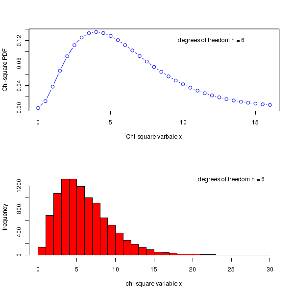
##### Using R library functions for Chi-square distribution
## Probability density for a given x, from a distribution with given degrees of freedom:
prob_dens = dchisq(x=6, df=5)
prob_dens = format(prob_dens, digits=4)
print(paste("Chi-square probability density for x=6, df=5 is = ", prob_dens))

## Cumulative probability upto x=6 for a Chi-square pdf with the given degrees of freedom.
cum_prob = pchisq(q=6, df=10)  ## function uses 'q' for x value
cum_prob = format(cum_prob, digits=4)
print(paste("chi-square cumulative probability upto x=6 for degrees of freedom 10 is  =  ", cum_prob))

## The value of variable x upto which the cumulative probability is p, for a
## chi-square distribution with given degrees of freedom
x = qchisq(p = 0.85, df=6)
x = format(x, digits=4)
print(paste("value x at which cumulative probability is 0.85 for 6 degrees of freedom = ",x))

## Generate 5 random deviates from a chi-square distribution with degrees of freedom 10
print(rchisq(n=6, df=10))


## we will draw 2 graphs on the same plot

par(mfrow=c(2,1))

## Drawing a chi-square distribution pdf in x = 0 to 12, with df=6
x = seq(0,16, 0.5)
chisq_pdf = dchisq(x, df=6)
plot(x, chisq_pdf, col="blue", type="b", xlab="Chi-square varbale x", ylab="Chi-square PDF")
text(12.0, 0.12, "degrees of freedom n = 6 ")

## Plotting the frequency histogram of gamma random deviate for shape=4, scale=1
hist(rchisq(n=10000, df=6), breaks=30, col="red", xlab="chi-square variable x",                             ylab="frequency",main = " ")
text(25, 1300, "degrees of freedom n = 6")
Executing the above code prints the following lines and displays the following plots on the screen :
[1] "Chi-square probability density for x=6, df=5 is =  0.0973"
[1] "chi-square cumulative probability upto x=6 for degrees of freedom 10 is  =   0.1847"
[1] "value x at which cumulative probability is 0.85 for 6 degrees of freedom =  9.446"
[1] 11.806898 10.434803  9.081138 13.650395 10.391160 17.583303