CountBio
Mathematical tools for natural sciences
Basic Statistics with R
Gamma distribution
In the previous section, we learnt that the waiting time until the first event in a Poission process follows an exponential distribution. Now we are interested in the waiting time \(\small{W}\) until certain number of events arrive.
let \(\small{W}\) be the waiting time until \(\small{\alpha}\) events arrive in a Poisson process with parameter \(\small{\lambda}\) (mean number of events per unit time). What will be the distribution of the continuous variable \(\small{W}\)?
Since the mean number of events that arrive in a time interval \(\small{w}\) is \(\small{\lambda w}\), we can write the Poisson probability for the arrival of \(\small{k }\) events in time \(\small{w}\) as \(\small{ \dfrac{(\lambda w)^k {\large e}^{-\lambda w}}{k!} }\)
For the arrival of \(\small{\alpha}\) events, we write the cumulative probability of having a waiting time upto \(\small{w}\) as,
\(~~~~~~~~\small{g(w)~=~P(W \leq w) = 1 - P(W \gt w)}\)
\(\small{~~~~~~~~~~~~~~~~~~~~~~~~~~~~~~~~~~~~~~=~1 - P(fewer~than~\alpha~events~arrive~in~interval~[0,w])} \)
\(\small{~~~~~~~~~~~~~~~~~~~~~~~~~~~~~~~~~~~~~~=~1 - \sum\limits_{k=0}^{\alpha-1} \dfrac{(\lambda w)^k {\large e}^{-\lambda w}}{k!} }\)
The probability distribution function (pdf) is the derivaive of the cumulative probability function. Skipping the inermediate steps, we directly write the derivative of cumulative probability distribution as,
The above expression gives the probability of waiting time \(\small{w}\) until the arrival of \(\small{\alpha}\) events in a Poisson process in which the mean number of events per unit time is \(\small{\lambda}\)
The above probability distribution is said to be of Gamma distribution . This name is derived from the gamma function defined by,
\(~~~~~~~~~~~~~~~~~\small{\Gamma(t) = \int\limits_0^\infty y^{t-1}e^{-y}dy~~~~~~~~~~~~t \gt 0}\)
The gamma function has an important property : \( \small{~~~~~\Gamma(n) = (n-1)! } \)
Using this result in the pression of \(\small{P_g}\) given above and letting \(\small{\theta = \dfrac{1}{\lambda} }\) and \((\alpha-1)! = \Gamma(\alpha) \), we get the pdf of gamma distribution as,
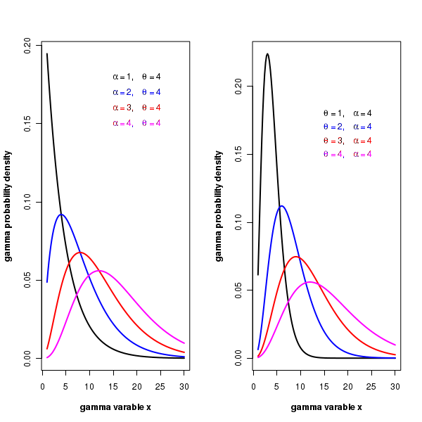
The plot of the gamma distribution
R-scripts
R provides functions for computing gamma distribution with probability density \(~~~~~~~~~~~~~~~~\small {f(x) = \dfrac{1}{\Gamma(\alpha) \theta^\alpha} {\large x}^{\alpha-1}{\large e}^{-x/\theta},~~~~~~~~~~~0 \leq x \lt \infty }\) where \(\small{\alpha}\) is the scale parameter and \(\small{\theta}\) is the shape parameter.
 dgamma(x, shape, scale) --------------> returns the gamma probability density for a given x value, shape and
                                            scale parameters

 pgamma(x, shape, scale) --------------> returns the cumulative probability from 0 upto x from a
                                            gamma distribution with the given shape and scale paramters.


 qgamma(p, shape, scale) ---------------> returns the  x value at which the cumulative probability is p from a
                                               gamma distribution with the given scale and shape parameters.

 rgamma(n, shape, scale) ---------------> returns n random numbers in the range [0 , infinity] from a
                                            gamma distribution with the given scale and shape parameters.


The R script below demonstrates the usage of the above mentioned functions:
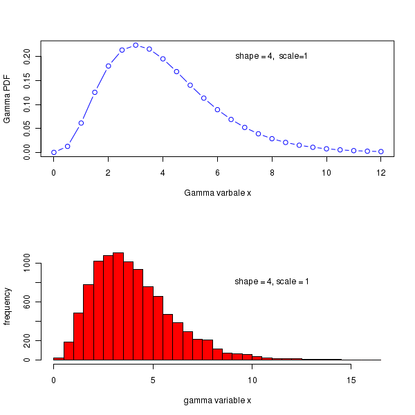
##### Using R library functions for Gamma distribution
## Probability density for a given x, from a distribution with shape and scale values:
prob_dens = dgamma(x=6, shape=4, scale=1)
prob_dens = format(prob_dens, digits=4)
print(paste("Gamma probability density for x=6, scale=4, shape=1 is = ", prob_dens))

## Cumulative probability upto x=6 for a gamma pdf with the given scale and shape values.
cum_prob = pgamma(q=6, shape=4, scale=1)  ## function uses 'q' for x value
cum_prob = format(cum_prob, digits=4)
print(paste("gamma cumulative probability upto x=6 for scale=4, shape=1 is  =  ", cum_prob))

## The value of variable x upto which the cumulative probability is p, for a
## gamma distribution with given shape and scale parameters
x = qgamma(p = 0.85, shape=4, scale=1)
x = format(x, digits=4)
print(paste("varable x at which cumulative probability is 0.85 is  =  ", x))

## Generate 5 random deviates from a gamma distribution with parameters shape=4, scale=1
print(rgamma(n=6, shape=4, scale=1))


## we will draw 2 graphs on the same plot

par(mfrow=c(2,1))

## Drawing a gamma distribution pdf in x = 0 to 12, with scale=1, shape=4
x = seq(0,12, 0.5)
gamma_pdf = dgamma(x, shape=4, scale=1)
plot(x, gamma_pdf, col="blue", type="b", xlab="Gamma varbale x", ylab="Gamma PDF")
text(8.0, 0.2, "shape = 4,  scale=1")

## Plotting the frequency histogram of gamma random deviate for shape=4, scale=1
hist(rgamma(n=10000, shape=4, scale=1), breaks=30, col="red", xlab="gamma variable x", ylab="frequency",
      main = " ")
text(11, 800, "shape = 4, scale = 1")
Executing the above code prints the following lines and displays the following plots on the screen :
[1] "Gamma probability density for x=6, scale=4, shape=1 is =  0.08924"
[1] "gamma cumulative probability upto x=6 for scale=4, shape=1 is  =   0.8488"
[1] "varable x at which cumulative probability is 0.85 is  =   6.014"
[1] 1.593189 2.012809 2.392053 2.754715 2.400868 3.282750