CountBio
Mathematical tools for natural sciences
Basic Statistics with R
Error bars in plots
Generally we plot the values of a dependent variable Y for various values of independent variable X as points (x_i,~y_i). For a given \(\small{x_i }\), the \(\small{y_i }\) is usually obtained as a mean value of n repeat measurements with a sample standard deviation \(\small{s_i }\). If the uncertainity on each value of Y is known, we should represent it as an error bar on the Y value. An error bar is a small segment of vertical line around each point (X,Y) which represent the uncertainity on the measured value Y. [ It should be called "uncertainity bar", since it represents the uncertainity in the data. Traditionally, it is called an "error bar"].
The vertical error bar on a point (x_i,~y_i) may represent any one of the following three quantities that quantify the spread in the data: \(~~~~~~~~~~~~~~~(i)~~\) The standard deviation \(\small{\sigma_{y_i} }\) (if known) or \(\small{s_{y_i} }\) \(~~~~~~~~~~~~~~(ii)~~\) The standard error on the mean \(\small{\dfrac{\sigma_{y_i}}{\sqrt{n}}~~ }\), where n is the number of samples used to determine the value Y. If \(\small{\sigma_{y_i} }\) is not known, we can use the estimate \(\small{ \dfrac{s_{y_i}}{\sqrt{n}} }\) \(~~~~~~~~~~~~~(iii)~~\) The confident interval around the (unknown) population mean given by \(\small{Z_{1-\alpha/2 } \dfrac{\sigma_{y_i}}{\sqrt{n} } ~~}\). If \(\small{\sigma_{y_i} }\) is not known, we can use \(\small{t_{1-\alpha/2 } \dfrac{s_{y_i}}{\sqrt{n} } }\). Usually a \(\small{95\% }\) confidence interval (\(\small{\alpha=0.05 }\) is chosen.
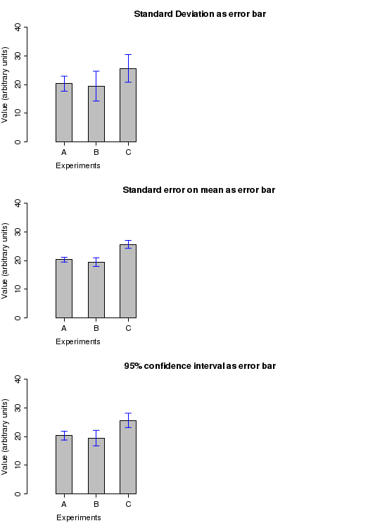
The Error Bars on a barplot
Let us consider the following three data sets A,B and C with unequal number of data points: \(\small{A~=~\{23.3, 20.0, 20.2, 15.3, 17.7, 23.1, 19.9, 20.2, 23.9, 19.8 \} }\) \(\small{B~=~\{ 10.1, 14.9, 17.3, 18.2, 27.2, 26.4, 15.4, 22.0, 24.2, 18.0, 23.9, 16.3 \} }\) \(\small{C~=~\{24.9, 15.6, 25.7, 25.0, 33.7, 23.9, 20.2, 30.7, 24.3, 25.8, 30.8, 27.6 \} }\) We compute : The sample sizes: \(\small{~~~~n_A = 10,~~~n_B = 12,~~~n_C = 12 }\) Sample means : \(~~~\small{\overline{x}_A = 20.34,~~~\overline{x}_B = 19.49,~~~\overline{x}_C = 25.68} \) Standard deviations : \(~~~\small{s_A = 2.62,~~~s_B = 5.22,~~~s_C = 4.83 }\) Standard error on mean : \(\small{SEM_A = \dfrac{s_A}{\sqrt{n_A}} = 0.83,~~~~SEM_A = \dfrac{s_B}{\sqrt{n_B}} = 1.51,~~~~SEM_C = \dfrac{s_C}{\sqrt{n_C}} = 1.39,~~~~}\) Next we compute the \(\small{95\% }\) confidence interval for the three samples. Since we are using the sample standard deviations, we should use t statistic for the confidence intervals. We have, For sample A, \(~~~\small{t_{0.95}(n-1) = t_{0.95}(9) = 1.83 }\) For sample B, \(~~~\small{t_{0.95}(n-1) = t_{0.95}(11) = 1.79 }\) For sample C, \(~~~\small{t_{0.95}(n-1) = t_{0.95}(11) = 1.79 }\) With this, the \(\small{95\% }\) confidence interval for A \(~~=~~\small{\overline{x}_A~\pm~t_{0.95}(n-1) \dfrac{s_A}{\sqrt{n_A}} ~=~20.34~\pm~1.83 \times \dfrac{2.62}{\sqrt{9} }~=~20.34~\pm~1.52 }\) the \(\small{95\% }\) confidence interval for B \(~~=~~\small{\overline{x}_B~\pm~t_{0.95}(n-1) \dfrac{s_B}{\sqrt{n_B}} ~=~19.49~\pm~1.79 \times \dfrac{5.22}{\sqrt{11} }~=~19.49~\pm~2.71 }\) the \(\small{95\% }\) confidence interval for C \(~~=~~\small{\overline{x}_C~\pm~t_{0.95}(n-1) \dfrac{s_C}{\sqrt{n_C}} ~=~25.68~\pm~1.79 \times \dfrac{4.83}{\sqrt{11} }~=~25.68~\pm~2.50 }\) The standard deviation, standard error or the confidence intervals are plotted as "error bars" around the data points on the bar plot as well as on the normal (X,Y) plots. First plot the mean value as a data point. Draw a vertical line segment above and below the mean point whose length is equal to the value of the error considered. The figure below shows the above mentioned three errors plotted as error bars for the data described above:
R scripts
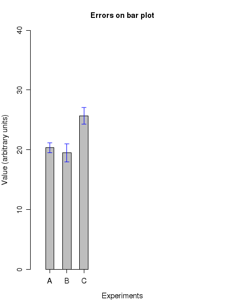
We can add error bars to the points in R plots. This is done in two steps. First draw a point or barplot, and then draw a vertical line segment in up and down direction from the point. The length of the segment is equal to the error value at that point. In the case of bar plot, draw the error bar in the middle of the top edge of the bar.
After the plot call, the function arrows() is called with the fiollowing parameter list:arrows(x0, y0, x1, y1, length, angle, code = 2, col, lty, lwd ) This function draws an arrow from point (x0, y0) to (x1,y1) in the same coordinate system as the plot() or barplot() functions. The various parameters are described here: (x0, y0) -------------> The start point of the arrow. (x1, y1) -------------> The end point of the arrow. length -------------> The length of the arrow head in inches angle -------------> Angle between arrow shaft and arrow head in degrees code -------------> Integer code that decides the type of arrow to be drawn. code=1 draws arrow head at start point, code=2 draws at end point and code=3 draws arrow head at both points. col, lty lwd ---------------> color, libe type and line width. Usual parameters of plot. The R script given below plots error bars on a barplot as well as on a (X,Y) plot.
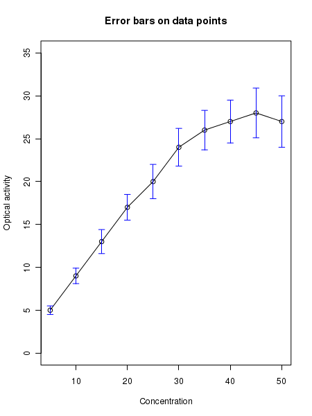
## error bars on bar plots

## mean values
means = c(20.34, 19.49, 25.68)

## standard errors
stderr = c(0.83, 1.51, 1.39)

## plot the bars
means_barx = barplot(means, names.arg=c('A','B','C'),ylim=c(0,40), axis.lty=1,
                   xlab="Experiments", ylab="Value (arbitrary units)", width=0.5,
		   xlim=c(0,10), space=1.0, col="grey",font.lab=1,
		    main="Errors on bar plot", cex.lab=1.2, cex.axis=1.2, cex.names=1.2,
		    cex.main=1.2 )

## Plot the up and down arrows as error bars on the bars
arrows(means_barx, means+stderr, means_barx, means-stderr, angle=90, code=3,
       length=0.06, col="blue")


X11()


### error bars on (x,y) points

## X and Y values of data points
x = c(5, 10, 15, 20, 25, 30, 35, 40, 45, 50)
y = c(5, 9, 13, 17, 20, 24, 26, 27, 28, 27)

## errors on Y values of individual data points. Generally, standard error on mean.
errors = c(0.5, 0.9, 1.4, 1.5, 2.0, 2.2, 2.3, 2.5, 2.9, 3.0)

## Plot the points first.
plot(x,y, ylim=c(0,35), type="o", xlab="Concentration", ylab="Optical activity",
     main="Error bars on data points")

## draw arrows up and down of data points to show the error bars.
arrows(x, y+errors, x, y-errors, angle=90, code=3, length=0.06, col="blue")
Running the above code creates the following two plots on the screen: