CountBio

Introduction to hypothesis testing

Introduction

The data points obtained from repeating an experiment or observation are assumed to have randomly sampled from a parent population also called as "parent distribution". From this sample data, we compute the sample parameters like sample mean, sample variance, etc.

Even before performing an experiment, we would come up with few statements on the population based on our prior knowledge about it. We belive that these statements are possibly true, and decide to perform experiments to test their validity. A statement on the population believed to be possibly true is called a hypothesis . Generally a hypothesis concerns the parameters of a population. For example, we want to compare the yields of two varieties of rice. Based on some prior knowledge, we make a hypothesis that the mean yield measured in units of Kg per acre of the two varieties are equal under some conditions. This is a statement on their population means. We then plant the two varities on a large area divided into many one acre patches and get their mean yields under the same conditions of our assumption. These sample means can then be used to check the validity of our hypothesis on the equality of the population means . This is how we can test our hypothesis.

We will illustrate the methodology of hypothesis testing with the following example:

An agricultural farm has been growing and selling medium sized water melons for many years. They have been measuring and noting down the weight of each pumpkin they harvested be before it goes to the market. Based on data on few hundred thousand pubpkins, they estimate a mean weight to be \(\small{2.35~Kg}\) with a standard deviation \(\small{0.36~Kg}\).

Now the form wants to test a new manure from a fertilizer company which is supposed to increase the yield of pubpkins significantly. To test this claim, the following experiment was devised. One fraction of the watermelon plants in the farm were treated with the new manure and the other plants were fed with the ususal fertilizer. At the end of the season, 100 pumpkins that grew with new manure were harvested and their mean weight was measured to be \(\small{2.46~Kg}\).

From this data, can we say whether the use of new fertilizer has considerably increased the pumbkin weight? What number we will use for this?

We will make use of the central limit theorem to analyse this data.

Suppose we assume that the weight of the particular variety of pumpkin that has been grown all these days in the farm without manure follows a Normal distribution with a mean \(\small{2.35~Kg}\) and a standard deviation of \(\small{0.36~Kg}\).

We also assume that the manure has not at all improved (changed) the yield of pumpkin when compared to yields of previous ones without menure. Then, the 100 pubpkins grown with manure are also can be considered to be the random samples from the above mentioned gaussian whose population mean is \(\small{\mu = 2.35~Kg}\) and standard deviation \(\small{\sigma = 0.36~Kg}\).

The estimated mean (sample mean) of these 100 pumbpkins turns out to be \(\small{\overline{X} = 2.46~Kg }\). This is the mean weight of 100 random samples from our Gaussian distribtuion.

We know that this sample mean \(\small{\overline{X} }\) should follow a Normal distribution according to central limit theorem. Thus we can write,

\(\small{Z = \dfrac{\overline{X} - \mu}{\left(\dfrac{\sigma}{\sqrt{n}}\right)} = N(0,1) ~~ }\) a unit normal distribution.

Substituting \(\small{\overline{X} = 2.46 }\), \(\small{\mu = 2.35 }\), \(\small{\sigma = 0.36 }\) and \(\small{n = 100 }\) in the above expression for Z, we get

\(\small{Z = \dfrac{2.46 - 2.35}{\left(\dfrac{0.36}{\sqrt{100}}\right)} \approx 3.055 }\)

Since Z follows a unit normal distribution, the probability of having \(\small{Z > 3.055 }\) is same as the probability of having a weight greater than \(\small{2.46~Kg }\) in a Normal distribution with mean \(\small{\mu = 2.35~Kg}\) and standard deviation \(\small{\sigma = 0.36~Kg}\).

The R function call 1 - pnorm(3.055) returns this probability to be 0.001125 .

What does this probability 0.001125 mean?.

Under the assumption that the new menure does not increase the yield (ie., yield remains same as before), the probability that the mean yield of 100 random samples (grown on menure) can be greater than \(\small{2.46~Kg }\) is 0.001125.

We take 100 random samples and find the mean. If we repeat this experiment 1000 times, approximately once we will get a mean value greater than 2.46 Kg (or, equivalently, Z > 3.055).

Thus, under the assumption of menure having no effect on yield, the chance probability of getting the observed mean of 2.46 with 100 random samples from a Normal distribution \(\small{\mu=2.35, \sigma=0.36 }\) is 0.001125.

Suppose we declare that this chance probability of 0.001125 ( a probability of approximately 1 in 1000) is very small. This implies that the event in which our 100 samples giving a mean yield of 2.46 Kg is rare. This in turn implies that the increase in mean yield from expected parent mean of 2.35 Kg to the observed 2.46 Kg may be due to the action of new manure. This is not directly proved. The rarer the chance of occurance by nature, more probable that it is due to the other cause.

To conclude, we have demonstrated the following in our experiment: We knew that the yield follows a Gaussian with a given mean and sigma. Under the assumption of no effect, the probability of observing the sample mean in this Gaussian distribution is 0.001125, which we feel is very small, and hence a rare event. Therefore, within this definition of rarity, we conclude that the observed mean of 100 samples support the fact that the menure has increased the yield considerably to a level which is not easy to observe normally by chance in the parent distribution. This fact is against our assumption that the manure does not affect the yield.

The steps of hypothesis testing

The whole exercise described above is called hypothesis testing . We will now formally describe the steps with technical terms.

1. Data collection : The first step is to collect the data from the experiment. In this case, the weights of 100 randomly selected water melons grown with new manure is the data. We also collect the additional information that the population mean is \(\small{2.35~Kg }\) with a standard deviation of \(\small{0.36~Kg. }\)

2. Assumptions on data and the underlying distribution : We make several assumptions about the nature of the data. Sometimes, the methods of analysis depends of these assumptions. For example, we want to make sure that the data points within a data set are independent. We also should know whether the two data samples we compare are dependent or independent samples. Also, we should make a reasonable assumption on the nature of the distribution of the population from which the data points are assumed to have been randomly drawn during the experiment. We should also make assumptions about the equality of means and variances, if we compare more than one distribution.

In the current problem, we assumed that the weights of individual water melons are independent, and follow a Gaussian distribution with mean and standard deviation based on very large number of samples. How do we know that the weights follow Gaussian?. We might plot a histogram of very large number of water melons to verify this. Even if the distribution is not exactly Gaussian, we can make use of central limit theorem to get a probability.

2. State the hypothesis : In the above analysis, we wanted to find out whether the new manure increase the yield. We set about testing the statement that "the menure does not increase the yield". This is called a null hypothesis which is generally a hypothesis of no change . The null hypothesis in general is opposite of what we want to find out. It is generally set up in such a way that if our data defeats(rejects) the null hypotheis, we get the desired effect. In this case, the rejection of null hypothesis means that the menure increases the yield . This is the alternate hypothesis.. Thus the alternate hypothesis is our desired effect, and null hypothesis is the no effect statement. (Note: it can be stated otherway around also, but this is the general procedure). If null hypothesis is accepted in the end, we see no effect. If null hypothesis is rejected and alternate hyopothesis is accepted, we obseve the desired effect in the data.

The symbol \(\small{H_0 }\) is used to represent the null hypothesis, and \(\small{H_A}\) for alternate hypothesis. Let us assume that the n measurements of menure treated yields are random samples from a Gaussian whose mean is \(\small{\mu }\) with standard deviation \(\small{\sigma}\). We have already assumed that the untreated yields follow a Gaussian distribution with mean \(\small{\mu_0 = 2.34}\) and standard deviation \(\small{\sigma=0.36}\).

In the current problem, we state the null hypothesis that the population mean \(\small{\mu }\) of the menure treated yield is same as or less than the non-menure treated population mean and has not increased. We can thus write the null and alternate hypothesis for this problem as,

\(~~~~~~~~~~~~~~~\small{H_0 :~\mu \leq \mu_0 }\)
\(~~~~~~~~~~~~~~~\small{H_A :~\mu \gt \mu_0 }\)

3. Define the test statistic and its distribution : The next step is to define a suitable statistic with which we can test the null hypothesis. For this data, we can calculate a mean \(\small{\overline{x}}\) for n random samples with manure. Under the null hypothesis, since the manure has no effect, these n samples are assumed to have been from a Gaussian distribution of mean \(\small{\mu_0}\) and standard deviation \(\small{\sigma }\). If this is true, according to central limit theorem, the statistic,

\(\small{Z = \dfrac{\overline{X} - \mu_0}{\left(\dfrac{\sigma}{\sqrt{n}}\right)} ~~}\) should follow N(0,1), a unit normal distribution.

4. Define a level of acceptance and a decision rule : For a particular value of \(\small{\overline{X},\mu, \sigma}\) and n, we compute a Z. Under the null hypothesis, this Z should have been randomly drawn from a unit normal distribution \(\small{N(\mu_0, \sigma})\).

What is the probability of observing a value of statistic above this computed Z value in unit normal distribution?. We call this "p-value"

If this p-value is very small, then it is less probable that the data samples would have come from a normal distribution \(\small{N(\mu_0, \sigma )}\). It is even lesser probable that the samples would have been drawn from a distribution with mean \(\small{\mu \lt \mu_0 }\) This result is against our null hypothesis that the menure has no effect, ie., \(~~~~~~~~~~~~~~~\small{H_0 :~\mu \leq \mu_0 }\). We say that the null hypothesis is rejected or the alternate hypothesis is accepted .

On the other hand, suppose the computed p-value for the data turns out to be large. This means, the probability of getting the observed Z value in a unit normal is large which in turns implies that the menure has not appreciably increased the yield to make the observed data points very different from those sampled from \(\small{N(\mu_0, \sigma) }\). This is in agreement with our null hypothesis of menure not increasing the yield. We say that the null hypothesis is accepted or alternate hypothesis is rejected .

in order to decide whether the computed p-value is less ot more, we need a reference p-value to compare. This reference probabaility is called the level of statistical significance, denoted by the letter \(\small{\alpha}\).

Let \(\small{p}\) denote the computed p-value. Then we can write,

If \(~~\small{p \leq \alpha,~~}\), the null hypothesis \(~~\small{H_0 :~\mu \leq \mu_0 ~~ }\) is rejected and accept the alternate hypothesis.

If \(~~\small{p \gt \alpha,~~}\), the null hypothesis \(~~\small{H_0 :~\mu \leq \mu_0 ~~ }\) is accepted and reject the alternate hypothesis.

The above set of rules for the rejection or acceptance of null hypothesis are called decision rule .

What should be the value of \(\small{\alpha}\) used for the decision on p-value?. Thiis value is arbitrary. There is a general consensus in the scientific community that the value of \(\small{\alpha}\) should not exceed 0.05 on the higher side, while there is no limit on its value on the lower side. Thus the value of probability \(\small{\alpha }\) is in the range 0 to 0.05.

Smaller the value of \(\small{\alpha}\), more statistical significance is attached to the acceptance or rejection of the null hypothesis. Thus a hypothesis rejected with \(\small{\alpha=0.01}\) is considered to be more significant than the hypothesis rejected with \(\small{\alpha = 0.05}\). Smaller and smaller values of \(\small{\alpha}\) require more stronger effects to reject the null hypothesis. For a given problem studied, we cannot choose arbitrariely small values of \(\small{\alpha}\).

5. Critical value of test statistic : For a chosen value of \(\small{\alpha}\), we find the \(\small{Z_\alpha}\) value on the unit Gaussian such that the area under the curve above this value is \(\small{\alpha}\). This \(\small{Z_\alpha}\) is called critical value .

We can also make a decision rule based on critical value. For the Z value of current data set in the current problem,

reject the null hypothesis if \(\small{Z \geq Z_\alpha }~~~~~~~~~~\) (same as the decision rule \(\small{p~value \leq \alpha }\) )

accept the null hypothesis is \(\small{Z \lt Z_\alpha }~~~~~~~~~~\) (same as the decision rule \(\small{p~value \gt \alpha }\) )

We can reject or accept the null hypothesis using a decision rule with either p-value or the critical value.

6. Compute the test statistic and apply the decision rule : We already computed the test statistic Z for this problem:

\(\small{Z = \dfrac{2.46 - 2.35}{\left(\dfrac{0.36}{\sqrt{100}}\right)} \approx 3.055 }\)

Let us fix the level of significance at \(~~\small{\alpha = 0.05}\)

The p value for this Z statistic in a unit normal distribution is calculated using R function call,

\(~~~~~~~~~~~~\small{p = 1 - pnorm(3.055) = 0.001125}\)

Since \(\small{p \lt \alpha}\), the the null hypothesis is rejected .

Next, we find the critical value \(\small{Z_{0.95}}\) corresponding to the \(\small{\alpha = 0.05}\). The \(\small{Z_{0.95}}\) is located such that the area to the right of it is 0.001125 and the area to the left of it is (1-0.001125). Using the R function call

\(\small{Z_{1-\alpha} = Z_{0.95} = qnorm(0.95) \approx 1.6448~~~ }\) is the critical value.

Since the value 3.055 of the computed statistic of the data is to the right of critical value, we reject the null hypothesis and accept the alternate hypothesis to conclude that the population mean \(\small{\mu}\) of the data is greater than \(\small{2.35~Kg}\).

The one sided and two sided hypothesis

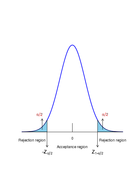
The rejection region in a hypothesis testing is decided by the question asked for the test. In general, there are three types of questions:

1. Can we conclude from the test that \(\small{\mu \neq \mu_0? }\)

In this case, the null and alternate hypothesis are given by,

\(~~~~~\small{H_0~:~\mu = \mu_0 }~~~~~~~~and~~~~~~~~~\) \(~~~~~\small{H_A~:~\mu \neq \mu_0 }\)

The null hypothesis can be rejected by values of statistic which are much larger than or much smaller than \(\small{\mu_0}\). In this case, the rejection region is split into two, one on each end of the ditribution.

Therefore, for a given significance of \(\small{\alpha}\), we choose two rejection regions, one on each tail such that the rejection area on each will be \(\small{\dfrac{\alpha}{2} }\). This is called two sided test . The acceptance and rejection regions of a two sided test are shown in the figure below:

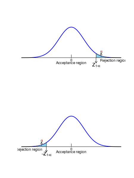
2. Can we conclude from the test that \(\small{\mu \gt \mu_0? }\)

The null and alternate hypothesis are,

\(~~~~~\small{H_0~:~\mu \leq \mu_0 }~~~~~~~~and~~~~~~~~~\) \(~~~~~\small{H_A~:~\mu \gt \mu_0 }\)

In this case, the null hypothesis is rejected by the sufficiently large values of the statistic. The whole of the rejection region will be on the higher end of the distribution tail with area \(\small{\alpha}\). This is also a one sided hypothesis testing .

3. Can we conclude from the test that \(\small{\mu \lt \mu_0? }\)

In this case, the null and alternate hypothesis are given by,

\(~~~~~\small{H_0~:~\mu \geq \mu_0 }~~~~~~~~and~~~~~~~~~\) \(~~~~~\small{H_A~:~\mu \lt \mu_0 }\)

This null hypothesis can be rejected by values of statistic which are sufficiently smaller. In this case, the whole rejection region is at one end of the distribution tail, with area \(\small{\alpha}\). This is also a one sided hypothesis testing .

The firgure below shows the regions of rejection for the one sided hypothesis testing: