CountBio

One sample t test

This test is applied to the case when we sample data points from a population which follows a normal distribution, or near normal distribution and the population varince is unknown.

The n data points \(\small{x_1,x_2,.....,x_n} \) are assumed to be the random samples from a Gaussian (or near Gaussian) distribution of mean \(\small{\mu}\) and a unknown standard deviation \(\small{\sigma}\).

When the population variance is unknown, the t statistic computed from the mean \(\small{\overline{x} }\) and standard deviation \(\small{s}\) of n random samples from a normal or near normal distribution follows a t distribution with n-1 degrees of freedom:
\(~~~~~~~~~~~~~~~~~~~~~ \small{t = \dfrac{\overline{x} - \mu}{\left(\dfrac{s}{\sqrt{n}}\right)} = t(n-1) }\)



We proceed with the hypothesis testing as follows:

• We first compute the sample mean \(\small{\overline{x}}\) from the data.


• Knowing the value of mean \(\small{\mu}\) and the computed standard deviation \(\small{s}\) of the sample, we compute the value of t using above expression.


• The statistical significance (also called "p-value") of this data is then obtained by computing the probability \(\small{P(\gt t) }\) or \(\small{P(\lt -t })\) from the t distribution. Under the null hypothesis, the p-value represents the probability of getting the observed statistic t.


• If the p-value is either smaller than a pre-decided value \(\small{\alpha}\) or the observed t statistic is outside a given range (\(\small{-t_0 \leq t \leq t_0) }\), we reject the null hypothesis and accept the alternate hypothesis.

Here, \(\small{t_0}\) is the value of statistic above which the area under the unit normal curve is \(\small{\alpha}\).


• We can also reject the null hypothesis if the computed t statistic for the data is outside the \(\small{(1-\alpha)100\%}\) confidence interval on the population mean.

Example-1 : Two sided hypothesis test

A sweet shop sells 100 gram packs of a variety of candy. In order to test the quality control of the packing process, a random sample of 16 packs were taken from the population consisting of very large number of packs and were weighed. The measurements in units of grams for each packet are given below:

\(\small{ 96.0,~~104.0,~~99.1,~~97.6,~~99.4,~~92.8,~~105.6,~~97.2,}\)
\(\small{96.8,~~92.1,~~100.6,~~101.5,~~100.7,~~97.3,~~99.6,~~105.9}\)

Assuming that the weights of individual packs follow a Gaussian, test whether the population mean of the pack weight is significantly different from 100 grams. Use \(\small{\alpha = 0.05}\) as the level of significance for rejecting the null hypothesis.


Since we want to test whether the population mean is not equal to 100, we set up the null and alternate hypothesis as follows:
\(~~~~~~~~~~~\small{H_0 : \mu = 100 } \)
\(~~~~~~~~~~~\small{H_A : \mu \neq 100}\)
Since the alternate hypothesis can be satisfied by the values greater than or less than the given \(\small{\mu}\) value, this is a two sided test.

Also,the population variance is not known. We use the t statistic for the test.

We first compute the mean and standard deviation of the sample. We get,
\(~~~~~~~~~\small{\overline{x} = 99.1,~~~~~~~~~~~~~s = 3.97}\)

Under null hypothesis, the t statistic should follow a t distribution with n-1 degrees of freedom. We compute the statistic from the data:

\( \small{t = \dfrac{\overline{x} - \mu}{\left(\dfrac{s}{\sqrt{n}}\right)} = \dfrac{99.1 - 100 }{\left(\dfrac{3.97}{\sqrt{16}}\right)} = -0.907 }\)

testing the null hypothesis using rejection regions:

We have taken \(\small{\alpha =0.05}\) to be the probability for rejecting the null hypothesis. Since the rejection can occur due to sufficiently small as well as large values of the test statistic, the rejection probability \(\small{\alpha =0.05}\) is divided equally between these two areas to give \(\small{\alpha/2 =0.025}\).

What is the t value for which the area above t or area below -t under the t distribution with n-1 = 15 degress of freedom is equal to \(\small{\alpha/2 =0.025}\)?. From the table of t distribution with 15 degrees of freedom, we read this to be approximately 2.13.

We reject null hypothesis if the computed test statistic t is either greater than 2.13 or less than -2.13. This rejection region is indicated as shaded portion in the figure below:

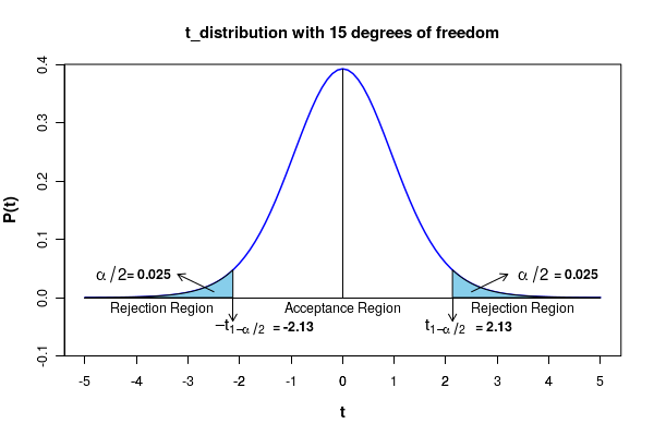
Since the computed value of t statistic t = -0.907 is in the acceptance region, we accept the null hypothesis to conclude that population mean of package weight is not significantly different from 100 grams. The statistical significance of this test is 0.05.

Testing the null hypothesis by computing the p-value for the observation:

If the null hypothesis is true, what is the probability of getting the computed t statistic?. This probability is called the"p-value" of the observed test statistic.

For the computed t value of -0.907, the p-value is obtained from the t distribution table corresponding to 15 degrees of freedom to be \(\small{p = 0.189 }\). This is the area under the curve to the left of \(\small{Z =-0.907 }\).

Since the p-value \(\small{p=0.189 }\) of the observed test statistic is more than \(\small{\alpha/2 = 0.025}\), we accept the null hypothesis to a significance level of 0.05.

In general, for a 2 sided test, we reject the null hypothesis if \(\small{p \leq \alpha/2 }\).
If \(\small{p \gt \alpha/2 }\), we do not reject the null hypothesis.

Testing the null hypothesis by computing the confidence interval:

For a significance level \(\small{\alpha = 0.05}\), the $95\%$ two sided confidence interval(CI) for the population mean is given by,
\(~~~~~~~~~~~~\small{CI~=~\overline{x} \pm t_{0.975} {\dfrac{s}{\sqrt{n}} }}\).
Substituting \(\small{\overline{x}=99.1,~~~~s=3.97,~~~~n=16}\) from the data and \(~\small{t_{0.975}(15)~=~2.13}~\) from the t table for 15 degrees of freedom, we get a $95\%$ confidence interval of \(\small{CI = 99.1 \pm 2.13*\dfrac{3.97}{\sqrt{16}}= 99.1 \pm 2.11 = (97.0, 101.2)}\)
Since this $95\%$ confidence interval \(\small{(97.0, 101.2)}\) contains the sample mean 99.1, we accept the null hypothesis at the level of 0.05 and conclude that the population mean for the weight of the pack is \(\small{\mu = 100~grams}\).

Example-2 : One sided hypothesis test

A chemical company was discharging a particular chemical wastse into a nearby river for many years. Based on very long term meansurements, the amount of waste product in the river water near the factory was estimated to be 480 in units of parts per million. With the tightening of environmental standards, the company decided to implement new methods in place to reduce this discharge into the river. Six months after implementation, 25 random samples of water was taken from the river at locations near the factory, and the amount of chemical in water were measured. Data is presented below:

348.3, 297.5, 225.5, 297.4, 328.8, 453.4, 219.7, 200.9, 549.4, 563.8, 366.9, 276.3,
471.7, 489.7, 241.6, 204.8, 335.2, 124.7, 575.6, 259.5, 519.6, 168.7, 301.6, 342.5, 333.2

To test whether the amount of waste product in the water has significantly reduced, we will perform a one sided test, using 0.01 as the level of sinificance. In the absene of information on the population vriance, we will use t statistic for the test.


We make the assumption that the amount of waste product in the samples collected from near locations come from a normal distribution.

The reduction of waste is tested by rejecting the null hypothesis when the mean value of the measurement is less than 480. Accordingly, the null and alternate hypothesis are stated as,

\(~~~~~~~~~~~\small{H_0 : \mu \geq 480 } \)
\(~~~~~~~~~~~\small{H_A : \mu \lt 480}\)





Testing the null hypothesis using rejection regions:



Though the null hypothesis is true for the infinite number of values of \(\small{\mu \leq 480}\), it is tested at only one value \(\small{\mu = 480 }\). If it is rejected at this value, it will be rejected at any lesser value.

From the data given above, we compute the value of sample mean and standard deviation:

\(~~~~~~~~~~~~~\small{\overline{x} = 339.8,~~~~~~~~~~~~~s = 129.3 }\)

Next step is to compute the t statisic with \(\small{\mu=480,~\overline{x}=339.8,~~\sigma=129.3,~~n=12}\):

\(~~~~~~~~~\small{t = \dfrac{339.8 - 480 }{\left(\dfrac{129.3}{\sqrt{25}}\right)}~ = ~ -5.42 }\)

Since this is a one sided test with \(\small{H_A : \mu \lt 480 }\), the null hypothesis is rejected by the values much smaller than the population mean 480.

With the the given level of significance 0.01, the rejection region lies to the left of \(\small{-t_{1-\alpha}(n-1) = -t_{0.99}(24) \approx -2.49 }\).

Since the computed t value lies in the rejection region, we reject the null hypothesis to conclude that the mean value of the waste product in the water is less than 480, to a significance level of 0.01. The rejection regions are marked below:

Testing the null hypothesis by computing the p-value for the observation:

Using the R function call pt(-2.49, 24) corresponding to 24 degrees of freedom, the are under the curve less than \(\small{t = -2.49}\) is computed as \(\small{7.2 \times 10^{-6} } \). Since this is less than \(\small{\alpha = 0.01 }\) for a one sided test, we reject the null hypothesis to the significant level of 0.01.



Testing the null hypothesis by computing the confidence interval:

For a significance level \(\small{\alpha = 0.01}\), the $99\%$ one sided confidence interval(CI) for the population mean is given by,
\(~~~~~~~~~~~~\small{CI~=~\overline{x} - t_{0.99} {\dfrac{\sigma}{\sqrt{n}} }}\).
Substituting \(\small{\overline{x}=339.8,~~\sigma=129.3~~n=24}\) from the data and \(~\small{t_{0.99}~=~2.49}~\) from Gaussian table, we get a $99\%$ confidence interval of \(\small{CI = 339.8 - 2.49 \times \dfrac{129.3}{\sqrt{25}}= 339.8 - 64.4 = (339.8, 275.4)}\)
Since this $99\%$ one sided confidence interval \(\small{(339.8,275.4)}\) does not contain population mean 480, we reject the null hypothesis that \(\small{\mu \geq 480}\) to a significance level of 0.01. We accept the alternate hypothesis that \(\small{\mu \lt 480}\).

R-scripts

The R script given below performs the one sample t test. Given a data set x that is assumed to be randomly drawn from a Gaussian distribution of population mean mu and standard deviation sigma, the function returns the conclusions of the test along with computed statistic values.

       one_sample_t_test(x, muzero, alpha, null) 

where

       x  = data vector

       muzero  = population mean for comparison
 
       alpha  = significane level

       null   = string value indicating type of null hypothesis.
      
  Possible values of variable null are:   "equal", "less_than_or_equal", "more_than_or_equal" 

The function returns a vector with two numbers :  (p value, t statistics) .

##################################################
## One sample t test

## x = vector of data samples, which are numbers
## muzero = population mean for comparison
## alpha = significance level for testing
## null = string with three possible values "equal", "greater_than_or_equal", "less_than_or_equal" for indicating whether the test is one sided or two sided.

one_sample_t_test = function(x, muzero, alpha, null  ){

 ## compute sample mean
 xbar = mean(x)

 ## comput sample standard deviation
 s = sd(x)


 ## get the sample size
 n = length(x)

 ## compute the t statistic
 t_statistic = (xbar - muzero)/(s/sqrt(n))

 ## compute the p-value
 pvalue = 1.0

 if(t_statistic > 0)
    pvalue = 1 - pt(t_statistic, n-1)

 if(t_statistic < 0)
    pvalue = pt(t_statistic, n-1)

 if(t_statistic == 0)
    pvalue = 0.5


 ## Perform the statitical test by comaring the computed t statistic with the 
 ##    critical value for various cases


 ### Case 1 : Null hypothesis that populatin mean equals a given value

 if(null == "equal")
 {
   t_critical = qt(1 - (alpha/2), n-1)

   print("################################################################")
   print("One sample t test : ")
   print(paste("sample size = ", n))

   if( (t_statistic > t_critical) | (t_statistic < -t_critical) )
   {
     print("One sample t test : ")
     print(paste("sample size = ", n))
     print(paste("Null hypothesis is rejected at the level of significance ", alpha/2))
     print(paste("Population mean not equal to ", muzero))
     print(paste("p value for the test = ", pvalue))
     print(paste("Value of t statistic = ", round(t_statistic, digits=2)))
     print(paste("Critical value of the test = ", round(t_critical, digits=2)))
     resultVec = c(pvalue, round(t_statistic, digits=2))
   }

   if( (t_statistic < t_critical) & (t_statistic > -t_critical) )
   {
     print("One sample t test : ")
     print(paste("sample size = ", n))
     print(paste("Null hypothesis is accepted at the level of significance ", alpha/2))
     print(paste("Population mean equal to ", muzero))
     print(paste("p value for the test = ", pvalue))
     print(paste("Value of t statistic = ", round(t_statistic, digits=2)))
     print(paste("Critical value of the test = ", round(t_critical, digits=2)))
     resultVec = c(pvalue, round(t_statistic, digits=2))
   }
  }



 #####  Case 2 : Null hypothesis that population mean is less than or equal to a given value 

 if(null == "less_than_or_equal")
 {
   t_critical = qt(1 - alpha, n-1)

   print("################################################################")
   print("One sample t test : ")
   print(paste("sample size = ", n))

   if( t_statistic > t_critical )
   {
     print("One sample t test : ")
     print(paste("sample size = ", n))
     print(paste("Null hypothesis is rejected at the level of significance ", alpha))
     print(paste("Population mean greater than ", muzero))
     print(paste("p value for the test = ", pvalue))
     print(paste("Value of t statistic = ", round(t_statistic, digits=2)))
     print(paste("Critical value of the test = ", round(t_critical, digits=2)))
     resultVec = c(pvalue, round(t_statistic, digits=2))

   }

   if( t_statistic <= t_critical )
   {
     print("One sample t test : ")
     print(paste("sample size = ", n))
     print(paste("Null hypothesis is accepted at the level of significance ", alpha))
     print(paste("p value for the test = ", pvalue))
     print(paste("Value of t statistic = ", round(t_statistic, digits=2)))
     print(paste("Critical value of the test = ", round(t_critical, digits=2)))
     resultVec = c(pvalue, round(t_statistic, digits=2))

   }
 }



 ###### Case 3 : Null hypothesis that the population mean is less than or equal to a given value.

 if(null == "greater_than_or_equal")
 {
   t_critical = qt(1 - alpha,n-1)

   print("################################################################")
   print("One sample t test : ")
   print(paste("sample size = ", n))

   if( t_statistic < t_critical )
   {
     print("One sample t test : ")
     print(paste("sample size = ", n))
     print(paste("Null hypothesis is rejected at the level of significance ", alpha))
     print(paste("Population mean is less than ", muzero))
     print(paste("p value for the test = ", pvalue))
     print(paste("Value of t statistic = ", round(t_statistic, digits=2)))
     print(paste("Critical value of the test = ", round(t_critical, digits=2)))
     resultVec = c(pvalue, round(t_statistic, digits=2))

   }

   if( t_statistic >= t_critical )
   {
     print("One sample t test : ")
     print(paste("sample size = ", n))
     print(paste("Null hypothesis is accepted at the level of significance ", alpha))
     print(paste("p value for the test = ", pvalue))
     print(paste("Value of t statistic = ", round(t_statistic, digits=2)))
     print(paste("Critical value of the test = ", round(t_critical, digits=2)))
     resultVec = c(pvalue, round(t_statistic, digits=2))

   }
 }


    return(resultVec)


 }  ## end of the function


###############------------------------------------------------

## Perform a sample test with the function

## define a data set
x = c(96.0,  104.0,  99.1,  97.6,  99.4,  92.8,  105.6,  97.2,
       96.8,  92.1,  100.6,  101.5,  100.7,  97.3,  99.6,  105.9)

## mean to be compared
muzero = 100

## alpha value
alpha = 0.05

## call the function. "res" is a vector with p-vlue and t value for the test.
res = one_sample_t_test(x, muzero, alpha, "equal")

print(res)

Executing the above script in R prints the following results and figures of probability distribution on the screen:

[1] "################################################################"
[1] "One sample t test : "
[1] "sample size =  16"
[1] "One sample t test : "
[1] "sample size =  16"
[1] "Null hypothesis is accepted at the level of significance  0.025"
[1] "Population mean equal to  100"
[1] "p value for the test =  0.199101040706245"
[1] "Value of t statistic =  -0.87"
[1] "Critical value of the test =  2.13"
>