CountBio
Mathematical tools for natural sciences
Basic Statistics with R
Poisson distribution
Some experiments involve counting the number of events occuring in a given interval. The interval in which eents are counted can be a physical space interval, time interval or event interval, as illustrated by the examples below:
- Counting the number of phone calls arriving between 9am and 11 am ( a 2 hour time interval) in a telephone exchange.
- Counting the number of atoms undergoing radioactive decay from a source every 4 minutes (time interval).
- Counting the number of trees per kilometer distance randomly grown by the side of a railway track ( a length interval).
- Counting the number of random misoccurances like single nucleotide polymorphisims in intervals of 1000 nucleotides (interval in a DNA sequence of nucleotides).
- Number of trees per square kilometer area of a wide forest. (area interval)
In these experiments, we consider the number of events occuring in a given interval .
Suppose we divide the time or event space into intervals of equal length \( \small{\Delta t }\) and count the number of random events \(\small{x}\) occuring in each interval. Let \( \small{x_1,x_2,x_3, ....} \) be the number of events occuring in various intervals of width \( \small{\Delta t }\).
We want to compute the probability \(\small{P(x)}\) of observing x discrete random events in an interval given the mean number of events observed in the same interval. For example, if 6 events are observed per hour on an average, what is the probability of observing 11 events per hour?. This \(\small{P(x)}\) follows a Poisson distribution, named after the great French mathematician and physicist Simeon Denis Poisson (1781-1840) .
In order to derive an expression for Poisson probability distribution, we have to make certain assumptions regarding the phenomenon in order to simplify the mathematics. The assumtions are listed below: Assumption 1 : The intervals in which the events counted are non-overlapping. Assumption 2 : The events occuring in these non-overlapping intervals occur independent of each other. Assumption 3 : We can always find a shorter interval such that the probability of two or more number of events occuring in this short interval is zero. (ie., we can find an interval in which only one event occurs on an average). Assumption 4 : The probability that an event occurs in an interval is directly proportional to the width h of the interval. This is the funcdamental assumption on Poisson process. Thus the probability of an event occuring in a short interval of length \(\small{h}\) is \(\small{\lambda h}\), where \(\small{\lambda}\) is the proportionality constant used as a parameter in Poisson process. According to this requirement, \(\small{\lambda}\) will represent the mean number of events occuring per unit interval. Because of these simplifying assumption, the process we describe will be an approximate Poisson process . In the approximate Poisson process, we can compute the probability of a certain number of events to occur in some unit interval given the mean number of events that occur in the same unit interval. An expression can be derived using the following argument:
Derivation of the Poisson porbability:
Let us consider an interval of length 1 ( fro, 0 to 1 in some unit). We subdivide this unit interval into \(\small{n}\) sub intervals, each of width \(\small{\dfrac{1}{n}}\)as shown in figure below:
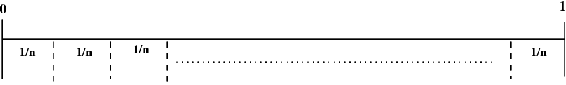
Consider \(\small{x}\) events occuring in this unit interval in a Poisson process. The division of unit interval into n sub-intervals is such that \(\small{n}\) is suffeciently larger than \(\small{x}\) and more than one event cannot occur in a sub-interval (see Assumption-3 above). Then, \(\small{P(x~events~in~an~unit~interval)~=~P(one~event~in~each~of~x~sub~intervals~of~width~\dfrac{1}{n}})\)
The probability of one event occuring in a sub-interval of width \(\small{\dfrac{1}{n}}\)is approximately \(\small{\lambda \times \dfrac{1}{n} }\), according to the Assumption-4 above. Therefore,
\(\small{P(one~event~occurs~in~any~one~of~n~sub intervals) = \dfrac{\lambda}{n}}\)
Since we have chosen the sub-interval such that only one event can occur, we can treat the occurance or non-occurance of an event in a sub-interval as a Bernoulli trial with \(\small{\dfrac{\lambda}{n}}\) as the probability of success.
Thus the probability of \(\small{x}\) events occuring in \(\small{n}\) sub-intervals (or, x events occuring in unit interval) is a Binomial probability \(\small{P_B(x, n, p)}\) with a probability \(\small{p=\dfrac{\lambda}{n}}\)for a single trial. Using the expression for Binomial probability, we write
$$\small{ P(x~events~in~n~sub~intervals) = \dfrac{n!}{x!(n-x)!}p^x (1-p)^{n-x} = \dfrac{n!}{x!(n-x)!}\left(\dfrac{\lambda}{n} \right)^x \left(1- \dfrac{\lambda}{n}\right)^{n-x} }$$
As n increases without bound, this probability reaches a limiting value at very very large \(\small{n}\). We can show that,
$$ \small{P(x) = \lim_{n\to\infty} \dfrac{n!}{x!(n-x)!}\left(\dfrac{\lambda}{n} \right)^x \left(1- \dfrac{\lambda}{n}\right)^{n-x} = } = \dfrac{\lambda^x e^{-\lambda}}{x!}~~~~~~~~~~~~~~~(derivation~not~shown~here) $$
We have thus derived the Poisson distribution which gives the probability of observing \(\small{x}\) events in an unit interval, where \(\small{\lambda}\) is the mean number of events in the same interval:
The Poisson variable \(\small{x}\) can take values from 0 to infinity in steps of 1, and the sum of probabilites of all possible values is exactly equal to 1. That is,
$$ \sum_{x=0}^{\infty} \dfrac{\lambda^x e^{-\lambda}}{x!} = 1 $$
The mean and the standard deviation of the Poisson distribution can be obtained as,
Thus the Poisson parameter \(\small{\lambda }\) which represents the mean number of events in unit interval turns out to be the mean \(\small{\mu}\) of the Poisson distribution, as expected. Also, we note this remarkable result : The mean \(\small{\mu}\) of a Possion distribution equals its variance \(\small{\sigma^2}\)
The expression for the probability density of Poisson distribution in terms of mean \(\small{\mu}\) is written as,
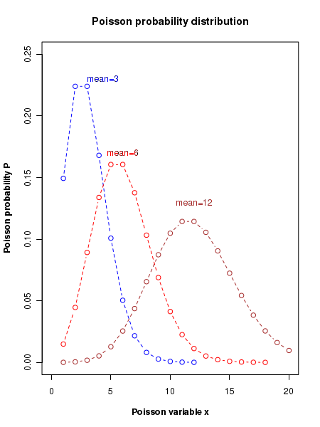
The plot of the Poisson distribution
The figure below displays the plots of Poisson distribution for various values of mean number of events \(\small{\mu}\) per unit interval. It should be noted that as the mean value increases, the distribution gets more and more symmetric about its peak value. For a mean value above 10, the shape of the distribution approaches a "bell shaped curve".
R scripts
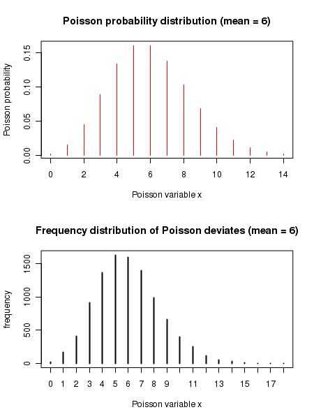
##### Using R library functions for Poisson distribution

## mu = mean number of events per unit intervel
## x = number of events in the same interval

## Computing Poisson probability density x given mean mu

mu = 10
x = 7
prob = dpois(x,mu)
prob = round(prob, digits=4)
print(paste("Poisson probability for x = ", x, "  mean = ", mu, " is ", prob))

### Function for computing cumulative probability.
### ppois(x,mu) gives cumulative probability for a Poisson distribution from 0 to x.
mu = 10
x = 7
cumulative_probability = ppois(x,mu)
cumulative_probability = round(cumulative_probability, digits=4)
print(paste("cumulative binomial probability for P(x=",x,",  mu=",mu,") = ",
                cumulative_probability) )

### Function for finding x value corresponing to a cumulative probability
mu = 10
cumulative_probability = 0.2202
x_value = qpois(cumulative_probability, mu)
print(paste("x value corresponding to the given  cumulative binomial probability ",
             cumulative_probability,"is ",x_value) )

### Function that returns 4 random deviates from a Poisson distribution of given mean

n = 4
mu = 10
deviates = rpois(n,mu)
print(paste("4 binomial deviates :  "))
print(deviates)


### We plot a Poisson density distribution using dpois()

par(mfrow=c(2,1))

mu = 6
x = seq(0,14)
pdens = dpois(x,mu)
plot(x,pdens, type="h", col="red", xlab = "Poisson variable x", ylab="Poisson probability",
     main="Poisson probability distribution (mean = 6)")

## We generate frequency histogram of binomial deviates using rbinom()
mu = 6
xdev= rpois(10000, mu)
plot(table(xdev), type="h", xlab="binomial variable x", ylab="frequency",
      main="frequency distribution of Poisson deviates (mean = 6)")
Executing the above script in R prints the following results and figures of probability distribution on the screen:
[1] "Poisson probability for x =  7   mean =  10  is  0.0901"
[1] "cumulative binomial probability for P(x= 7 ,  mu= 10 ) =  0.2202"
[1] "x value corresponding to the given  cumulative binomial probability  0.2202 is  7"
[1] "4 binomial deviates :  "
[1] 14 15  9 13