CountBio
Mathematical tools for natural sciences
Basic Statistics with R
Negative binomial distribution
Suppose we perform a sequence of Bernoulli trials and count the number of successess and failures. If \(\small{p}\) is the probability of success in any trial, how many trials we have to perform until we observe \(\small{r}\) successes?.
Here we are interested in a random variable \(\small{x}\) that represents the number of trials needed to observe the \(\small{r^{th}}\) success. Thus we may observe \(\small{r=5}\) successes in \(\small{x=8}\) trials or in \(\small{x=11}\) trials or in \(\small{x=9}\) trials. x is the trial number in which \(\small{r^{th} }\) success is observed, with \(\small{x \geq r }\). The observed values of the variable x follow the negative binomial distribution .
Another version of the negative binomial distribution is written in terms of the number of failures y before \(\small{r^{th}}\) success.
We will now derive expression for both the probability distribution for both the vairables \(\small{ x}\) and \(\small{ y}\) :
Derivation of the negative binomial probability: Version 1 : Number of trials \(\small{x}\) needed to observe \(\small{r^{th}}\) success. \(\small{P_{nb}(x,p,r) = P(x~trials~for~r~successes)}\) \(~~~~~~~~~~~~~~~~=~P(r-1~successes~in~the~first~x-1~trials) \times P(success~on~r^{th}~trial) \) We have, \( \small{P(r-1~successes~in~the~first~x-1~trials)~=~_{x-1}C_{r-1} p^{r-1} (1-p)^{x-r}~~~~~(binomial~distribution) }\) \(\small{P(success~on~r^{th}~trial) = p }\) We can thus write, \( P_{nb}(x,p,r) = \small{P(x~trials~for~r~successes)~=~_{x-1}C_{r-1} p^{r-1} (1-p)^{x-r} \times p~=~_{x-1}C_{r-1} p^{r} (1-p)^{x-r} } \)
Version 2 : Number of failures \(\small{y}\) before the \(\small{r^{th}}\) success.
Since \(\small{x }\) is the total number of trials before \(\small{r^{th}}\) success, \(~~~~\small{y = number~of~failures~before~r^{th}~success = x-r}\) We have,\(~~~~~~~~~ \small{P_{nb}(x,p,r)~=~_{x-1}C_{r-1} p^r (1-p)^{x-r} }\) Substituting from \(\small{y = x-r }\) for \(\small{x}\) in the above expression, we get \(~~~~~~~~~~\small{P_{nb}(y,p,r)~=~_{y+r-1}C_y p^r (1-p)^y }\)
The probability density functions for a negative binomial distribution for the number of trials \(\small{x}\) required for observing \(\small{r}\) successes and the number of failures \(\small{y}\) before the \(\small{r^{th}}\) success, with \(\small{p}\) being the probability of success in one trial, are summarised below. The mean and variance of these two variables are also given, without derivation:
Why is it called the "negative binomial" distribution?
For any real number \(\small{w}\), the expression \(\small{(1-w)^{-r} }\) with a negative exponent -r can be expanded as a sum using binomial theorem: \( \small{ (1-w)^{-r}~=~\sum\limits_{x=r}^{\infty} {_{x-1}C_{r-1}} w^{x-r} }\) The expression for the probability distribution given before is similar to the above negative binomial expansion except for the multiplicative constant \(\small{p^r}\). Hence the name negative binomial distribution .
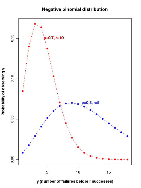
The plot of negative binomial probability distribution
The figure below displays the plots of negative binomial probability distribution for various values of probability \(\small{p}\) of success and the number of failures \(\small{r}\).
We will now learn to compute the negative binomial probability distribution in R
R scripts
The usage of these four functions are demonstrated in the R script here. With comments, the script lines are self explanatory:
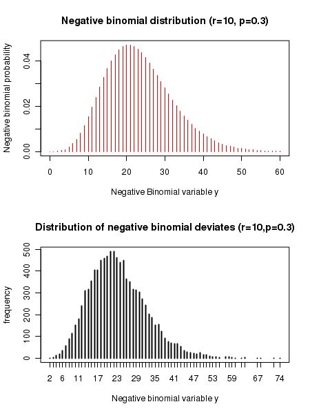
## Negative binomial distribution functions in R

## p = probability of success in a trial
## r = number of successes observed
## y = number of failures before r successes

## Computing negative binomial probability density for observing y failures before r successes:
y = 5
r = 3
p = 0.3
prob =  dnbinom(y, r, p)

print(paste("Negative binomial probability for " , y , " failures before " , r ,
               " successes is ",prob))


### Function for computing cumulative probability from x=0 to a given value.
### pnbinom(x,r,p) gives cumulative probability for a negative binomial distribution from 0 to x.
x = 5
cumulative_probability = pnbinom(x,r,p)
print(paste("cumulative negative binomial probability from x=0 to", x," for ", x,
              " failures before ",r, " successes is ", cumulative_probability) )

### Function for finding x value corresponing to a cumulative probability
cumulative_probability = 0.5
x_value = qnbinom(cumulative_probability, r, p)
print(paste("number of failures corresponding to the given  cumulative binomial
              probability of ", cumulative_probability," is ",x_value) )

### Function that returns 4 random deviates from a Negative Binomial distribution of given (n,p)
deviates = rnbinom(4, r, p)
print(paste("4 binomial deviates :  "))
print(deviates)


### We plot a binomial density distribution using dnbinom()
r = 10
p = 0.3
y = seq(0,60)
pdens = dnbinom(y,r,p)
plot(y,pdens, type="h", col="red", xlab = "Negative Binomial variable y",
         ylab="Negative binomial probability",
	 main="Negative binomial distribution (r=10, p=0.3)")

## We generate frequency histogram of binomial deviates using rbinom()
r = 10
p = 0.3
xdev= rnbinom(10000, r, p)
plot(table(xdev), type="h", xlab="Negative binomial variable y", ylab="frequency",
           main="Distribution of negative binomial random deviates (r=10,p=0.3)")
Executing the above script in R prints the following results and figures of probability distribution on the screen:
[1] "Negative binomial probability for  5  failures before  3  successes is  0.09529569"
[1] "cumulative negative binomial probability from x=0 to 5  for  5  failures before  3  successes is  0.44822619"
[1] "number of failures corresponding to the given  cumulative binomial probability of  0.5  is  6"
[1] "4 binomial deviates :  "
[1] 6 4 2 5