CountBio
Mathematical tools for natural sciences
Statistics for Machine Learning
Simple Linear Regression
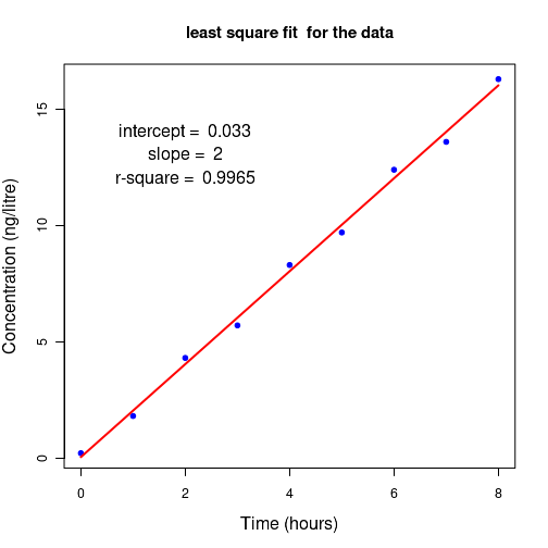
Suppose we perform an experiment to establish the relationship between two variables X and Y. We treat one of the variables (say X) as an independent variable and measure the values of Y for various values of X. The variable Y is called a dependent variable , since it is measured for a set of fixed values of X. The independent variable X is also called the predictor variable and Y the response variable . For example, in an experiment on laboratory mouse, we study the change in the concentration of blood sugar in response to the concentration of an infused drug in the blood. We mesure the concentration of blood sugar at various known concentrations of the drug in blood. Here, the medicine concentration is the indpendent(predictor) variable and the blood sugar measured is the dependent (response) variable. A set of data points between X and Y are shown in Figure-1 below:
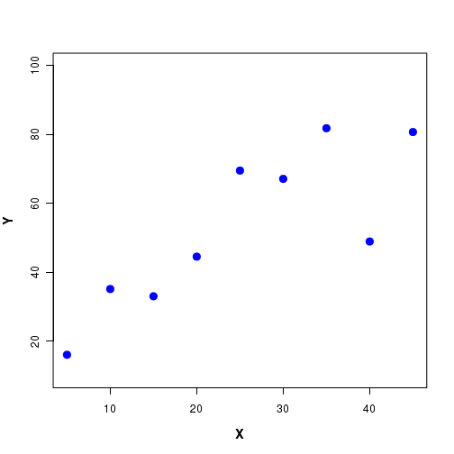
By looking at the scatterplot, suppose we decide that the relationship between X and Y can be approximated to be linear . We want to approximate the data points by a stright line of the form $y = a + bx$ so that for any given value of x in the data range, we can easily compute the approximate value of y from this equation. This is called a linear model for this data set.
By constructing this linear model, we replace a set of data points by the equation of a stright line through the points which approximately describes the relationship between X and Y in the given range of data. This helps us to qualitatively and quantitatively understand such a variation. Once the linear relationship is established, we can examine the inherent phenomena that result in a linear variation of Y as a function of X.
The problem is that infinite number of stright lines, each with a distinct slope and intercept, can pass through the given set of points. Three such lines are depicted in Figure-2 here:
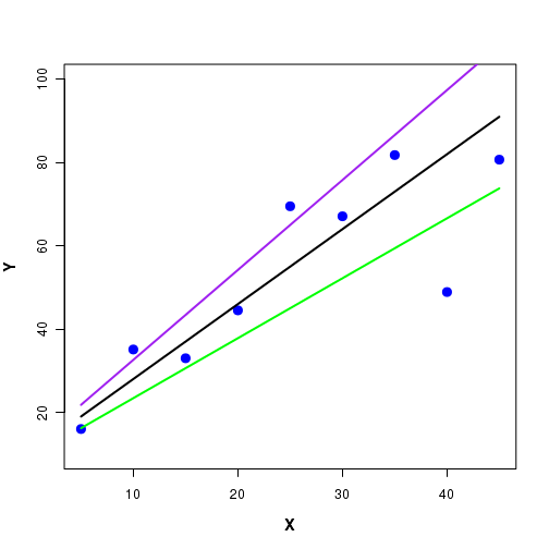
In the above Figure-2, we notice that each one of the three lines through the data lie close to some data points and far away from some other points. Infinite number of such lines are can pass through these data points. Which line is the best one?
The method of linear regression uses the observed data points to compute the slope and the intercept of the best straight line that can pass through the data points. The mathematical method is called the least square fit to a straight line . A straight line obtained from the observed data points (X,Y) using least square fit has the least deviation (error) between expected Y value on the line and the experimentally observed Y value for a given X value, when compared to any other line through the data points.
Important point : The method of least square fit to a stright line (linear regression) gives the best straight line through the data, with error minimized compared to any other line. It does not mean that such a line is the best curve through the data points. For example, for a given set of data points, the line obtained from least square method may have more error(deviations) from data points when compared to a polinomial of 5th degree obtained from least square fit of data to a polinomial!. Having decided to fit a curve (line strightline, exponential, polinomial etc) through the data point, the least square method gives the best curve (that minimized the error) in the family. If we decided to fit a strightline, we get the best stright line. If we decide to fit a parabola, we get the best parabola. Thus, for a given curve, the method of least squares gets the best parameters of the curve. If \(\small{y = mx+c}\) is the curve fitted, the method gives the best values for m and c that minimizes the error. Similarly, if \(\small{y = a_0 + a_1x^2 + a_2x^3 + a_3x^4}\) is the fitted curve, the method gives the best values for the coefficients \(\small{a_0, a_1, a_2, a_3 and a_4}\) that minimized the error. If we fit a straight line to a parabolic data points, we may still get the best stright line possible through the poins, but many points will deviate from the best fitted line!!. We will learn more on this later.
Before going into the procedure, we will list the assumptions underlying the liear regression:
Suppose, we denote the data points as ($x_1,y_1$), ($x_2,y_2$), ($x_3,y_3$), ...., ($x_n,y_n$).
1. The values of the independent variable X are fixed, and have no errors. X is a non-random variable.2. For a given value of X, the possible Y values are randomly drawn from a sub population of normal distribution. Thus, for a given value $x_i$ of X, observed $y_i$ is a point randomly drawn from a normal distribution. Also, the Y values for different X values are independent.
3. The means of the parent normal distributions from which the points $y_1, y_2,...,y_n$ were drawn lie on a straight line. The linear regression method in fact computes the slope and intercept of this (parent) straight line.. This can be expressed as an equation, $$ \mu_{y,x} = \beta_0 + \beta_1x$$ where $\mu_{y,x}$ is the mean value of the population from which the point y was drawn for the given x value. The coefficients $\beta_0$ and $\beta_1$ are called regression coefficients . 4. The variances of the parent normal distributions to which $y_1, y_2, ..., y_n$ belong can be assumed to be either equal or not equal in the derivation. Different expression will result based on these two assumptions. Regression analysis procedure
For the given data set (X,Y), let $y = \beta_0 + \beta_1x$ be the regression equation we want.
Since the we will never know the true regression coefficients, we will make an estimate of these coefficients from the data points. We name them $b_0$ and $b_1$ respectivly so that $y = b_0+b_1 x$ for the observed data set. The coefficients $b_0$ and $b_1$ estimated through regression theory are the best estimates of the original coefficients $\beta_0$ and $\beta_1$ respectively, which represent a staight line relation of population data.
For a given $x_i$, let the observed Y value be $y_i$. Then, $P_{obs}(x_i, y_i)$ will be this observed data point.
For a given $x_i$ value, let $y_i^{r}$ denote the corresponding point on this regression line. Then $P_{exp}(x_i, y_i^r)$ will be the expected data point on the regression line. See the Fifure-3 below:
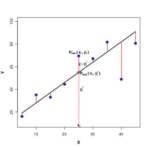
The linear regression procedure computes the square of the difference $(y_i - y_i^r)^2$ between the observed $y_i$ value and the expected $y_i^r$ value on the line for each data point. Using a minimization procudre, the sum of the squares of the differences $\sum(y_i - y_i^r)^2$ are minimized to get the coefficients $b_0$ and $b_1$.
For a given $x_i$, we have $y_i^r = b_0 + b_1x_i$. Using this, we can write the sum square normalized to the standard deviation as,
$$ \chi^2 = \sum_{i}\dfrac{1}{\sigma_i^2}(y_i - (b_0 + b_1 x_i) )^2$$By minimizing the above mentioned $\chi^2$ expression with respect to variables $b_0$ and $b_1$, we can get expressions for $b_0$ and $b_1$ in terms of observed data points ($x_i, y_i$). Using them we can compute $y_i = b_0 + b_1 x_i$ to plot the straight line through the data points.
See the box below for a complete derivation.
In the derivation, we consider two cases. The observed value $y_i$ is assumed to be a random sample derived from a Normal distribution $N(\mu_i, \sigma_i)$. In the first case, we assume that the standard deviations $\sigma_i$ are all equal. That is, all data points are drawn from distributions whose variances $\sigma_i$ are equal. In the second case, we assume that these variances $\sigma_i$ are unequal.
Derivation of linear regression coefficients: We start with our basic assumption that for a given independent variable $x_i$, the observed value $y_i$ follows a gaussian with mean $\mu_i = y(x_i) = b_0 + b_1x$ and standard deviation $\sigma_i$. For each point $(x_i, y_i)$, we write the Gaussian probability density as, \( ~~~~~~~~~~~~~~~\small{P(y_i|x_i, b_0, b_1, \sigma_i ) = \dfrac{1}{\sigma_i \sqrt{2\pi}} {\Large e}^{-\dfrac{1}{2}\left(\dfrac{y_i-y(x_i)}{\sigma_i}\right)^2} }\) where \(\small{P(y_i|x_i, b_0, b_1, \sigma_i )} \) is the probability of obtaining a $y_i$ given a value of $x_i$ and all the parameters of the model. The probability of observing n such independent data points is obtained by multiplying their individual probabilities. We denote this probability by $P(y|b_0,b_1,x)$. This is the "conditional probability of obtaining the data set y given the coefficients $b_0$, $b_1$ and the data set x". \(\small{P(y|b_0,b_1,x)}= P(y_1|x_1, b_0, b_1, \sigma_1 ) \times P(y_2|x_2, b_0, b_1, \sigma_2 ) \times .....\times P(y_n|x_n, b_0, b_1, \sigma_n ) \) \(~~~~~~~~~~~~~~~~~~~~~~\small{= \displaystyle\prod_{i=1}^{n} P(y_i|x_i, b_0, b_1, \sigma_i ) }\) \(~~~~~~~~~~~~~~~~~~~~~~\small{= \displaystyle\prod_{i=1}^{n} \dfrac{1}{\sigma_i\sqrt{2\pi}} {\Large e}^{-\dfrac{1}{2} \left(\dfrac{y_i-y(x_i)}{\sigma_i} \right)^2 } }\) \(~~~~~~~~~~~~~~~~~~~~~~\small{= \displaystyle\prod_{i=1}^{n} \dfrac{1}{\sigma_i\sqrt{2\pi}} {\Large e}^{-\dfrac{1}{2} \left(\dfrac{y_i-(b_0+b_1x_i)}{\sigma_i} \right)^2 } }\) The function $\small{P(y|b_0,b_1,x)}$ is called the "likelihood", a function of parameter values. Note that the data points $x_i$ and $y_i$ and $\sigma^2$ are constants from the data. Since the multiplication of exponential terms is equivalent to summing their exponents, we can write the above expression as, \(~~~~~~~~\small{ \small{P(y|b_0,b_1,x)}~=~\displaystyle{\left( \prod_{i=1}^{n} \dfrac{1}{\sigma_i\sqrt{2\pi}}\right)} ~ {\Large e}^{-\dfrac{1}{2} \displaystyle \sum_{i=1}^{n} \left( \dfrac{y_i-(b_0+b_1x_i)}{\sigma_i} \right)^2 } } \) The best values of $b_0$ and $b_1$ are the ones for which the above likelihood is maximum . Therefore we find the best fit values for the parameters by maximizing the likelihood function. This procedure is called method of maximum likelihood. Generally, the logarithms of the likelihood, called log likelihood is maximized to get the paramters. By looking at the expression we can realize that the probability is maximum when the negative exponent term given by, \(~~~~~~~~~~~~~~~~\small{\chi^2~=~\displaystyle\sum_{i=1}^{n} \dfrac{1}{\sigma_i^2} \left(y_i - b_0 - b_1x_i)^2 \right) }~~~~~~~\)is a minimum. The above term is called The least square sum . We have a data set with n date points (x_i, y_i) in which each $y_i$ is assumed to be randomly drawn from a Gaussian with mean $y(x_i) = b_0+b_1x_i$ and standard deviation $\sigma_i$. By minimizing the above least square sum with respect to the variable $b_0$ and $b_1$, we can obtain their best values for the data set. The line $y(x_i) = b_0 + b_1x_i$ is said to be the best fit to the data which minimizes the errors between observed $y_i$ values and the expected values $y(x_i)$ on the straight line. This procedure is also called as a least square fot to a straight line. The best fit valus for $b_0$ and $b_1$ are obtained by solving the equaltions, \( \dfrac{\partial \chi^2}{\partial b_0} = 0~~~~~~~~~and~~~~~~~ \dfrac{\partial \chi^2}{\partial b_1} = 0 \) At this stage, we consider two cases related to our assumption regarding the standard deviations:
Case 1 : The standard deviations $\sigma_i$ are all equal
We take the case for which \(\small{\sigma_1 = \sigma_2 = .....= \sigma_i = \sigma }\)
The expression for \(\small{\chi^2 }\) becomes,
\(~~~~~~\small{\chi^2 = \displaystyle\sum_{i=1}^{n} \dfrac{1}{\sigma^2}(y_i - b_0 - b_1x_i)^2 }\)
\(~~~~~~\small{~~~~= \dfrac{1}{\sigma^2}\displaystyle\sum_{i=1}^{n} (y_i - b_0 - b_1x_i)^2 }\)
Differentiating \(\small{\chi^2 }\) partially with respect to $b_0$ and $b_1$ and equating to zero, we get two equations:
\(\small{\dfrac{\partial \chi^2}{\partial b_0}~~=~~ \dfrac{-2}{\sigma^2} \displaystyle\sum_{i=1}^{n} (y_i - b_0 - b_1x_i)~~=~~0 }~~~~~~~~~~~~(1)\)
\(\small{\dfrac{\partial \chi^2}{\partial b_0}~~=~~ \dfrac{-2}{\sigma^2} \displaystyle\sum_{i=1}^{n} (y_i - b_0 - b_1x_i) x_i~~=~~0 }~~~~~~~~~~~~(2)\)
Equations (1) and (2) can be rearranged to get the following two simultaneous equations with $b_0$ and $b_1$ as variables:
\(\small{ \displaystyle\sum_{i=1}^{n} y_i~=~\displaystyle\sum_{i=1}^{n} b_0~+~\displaystyle\sum_{i=1}^{n} b_1x_i~=~ b_0n~+~b_1\displaystyle\sum_{i=1}^{n}x_i }~~~~~~~~(3)\)
\(\small{ \displaystyle\sum_{i=1}^{n}x_iy_i~=~ \displaystyle\sum_{i=1}^{n}b_0x_i~+~ \displaystyle\sum_{i=1}^{n} b_1 x_i^2~~=~~ b_0 \displaystyle\sum_{i=1}^{n}x_i~+~b_1 \displaystyle\sum_{i=1}^{n}x_i^2 }~~~~~~~~~~~~(4)\)
Solving the equations (3) and (4) for the variables $b_0$ and $b_1$, we get the following expressions for the coefficients of the least square fit for the case when all the data points have equal veriances. All the summations are over the index $i=1~to~n$, where n is the number of data points.
\(\small{
\Delta~=~
\begin{vmatrix}
n & \displaystyle\sum x_i \\
\displaystyle\sum x_i & \displaystyle\sum x_i^2 \\
\end{vmatrix}
~~=~~n \sum x_i^2 - (\sum x_i)^2
}\)
\(\small{
b_0~=~\dfrac{1}{\Delta}
\begin{vmatrix}
\displaystyle\sum y_i & \displaystyle\sum x_i \\
\displaystyle\sum x_i y_i & \displaystyle\sum x_i^2 \\
\end{vmatrix}
~~=~~\dfrac{1}{\Delta} \left(\sum y_i \sum x_i^2 - \sum x_i \sum x_i y_i\right)
}\)
\(\small{
b_1~=~\dfrac{1}{\Delta}
\begin{vmatrix}
n & \displaystyle\sum y_i \\
\displaystyle\sum x_i & \displaystyle\sum x_i y_i \\
\end{vmatrix}
~~=~~\dfrac{1}{\Delta} \left(n \sum x_i y_i - \sum x_i \sum y_i \right)
}\)
Case 2 : The standard deviations $\sigma_i$ are unequal
In this case, the standard deviations of populations from which $y_i$ were drawn are not equal. As a consequence, we cannot pull out the standard deviation term $\sigma_i$ out of the summations. We will go back to the derivation where we defined the Chi-square term:
\(~~~~~~~~~~~~~~~~\small{\chi^2~=~\displaystyle\sum_{i=1}^{n} \dfrac{1}{\sigma_i^2} \left(y_i - b_0 - b_1x_i)^2 \right) }~~~~~~~\) Now, differentiating with respect to the variables $b_0$ and $b_1$, we get \(\small{\dfrac{\partial \chi^2}{\partial b_0}~~=~~ -2 \displaystyle\sum_{i=1}^{n} \dfrac{1}{\sigma_i^2} (y_i - b_0 - b_1x_i)~~=~~0 }~~~~~~~~~~~~(5)\) \(\small{\dfrac{\partial \chi^2}{\partial b_1}~~=~~ -2\displaystyle\sum_{i=1}^{n} \dfrac{1}{\sigma_i^2}(y_i - b_0 - b_1x_i) x_i~~=~~0 }~~~~~~~~~~~~(6)\) Equations (5) and (6) can be rearranged to get the following two simultaneous equations with $b_0$ and $b_1$ as variables: \(\small{ \displaystyle\sum_{i=1}^{n} \dfrac{y_i}{\sigma_i^2}~=~ b_0 \sum \dfrac{1}{\sigma_i^2}~+~b_1\displaystyle\sum_{i=1}^{n} \dfrac{x_i}{\sigma_i^2} } ~~~~~~~~(7)\) \(\small{ \displaystyle\sum_{i=1}^{n} \dfrac{x_iy_i}{\sigma_i^2 }~=~ b_0 \displaystyle\sum_{i=1}^{n} \dfrac{x_i}{\sigma_i^2}~+~b_1 \displaystyle\sum_{i=1}^{n} \dfrac{x_i^2}{\sigma_i^2} }~~~~~~~~~~~~(8)\) Solving the above two equations for the variables $b_0$ and $b_1$, we get their expressions in terms of the data points $(x_i, y_i$ : \(\small{ \Delta~=~ \begin{vmatrix} \displaystyle\sum\dfrac{1}{\sigma_i^2} & \displaystyle\sum\dfrac{x_i}{\sigma_i^2} \\ \displaystyle\sum\dfrac{x_i}{\sigma_i^2} & \displaystyle\sum\dfrac{x_i^2}{\sigma_i^2} \\ \end{vmatrix} ~~=~~\displaystyle\sum\dfrac{1}{\sigma_i^2} \sum\dfrac{x_i^2}{\sigma_i^2} - \displaystyle\sum\dfrac{x_i}{\sigma_i^2} \sum\dfrac{x_i}{\sigma_i^2} }\) \(\small{ b_0~=~\dfrac{1}{\Delta} \begin{vmatrix} \displaystyle\sum \dfrac{y_i}{\sigma_i^2} & \displaystyle\sum \dfrac{x_i}{\sigma_i^2} \\ \displaystyle\sum \dfrac{x_i y_i}{\sigma_i^2} & \displaystyle\sum \dfrac{x_i^2}{\sigma_i^2} \\ \end{vmatrix} ~~=~~\dfrac{1}{\Delta} \left(\sum \dfrac{y_i}{\sigma_i^2} \sum \dfrac{x_i^2}{\sigma_i^2} - \sum \dfrac{x_i}{\sigma_i^2} \sum \dfrac{x_i y_i}{\sigma_i^2}\right) }\) \(\small{ b_1~=~\dfrac{1}{\Delta} \begin{vmatrix} \displaystyle\sum\dfrac{1}{\sigma_i^2} & \displaystyle\sum \dfrac{y_i}{\sigma_i^2} \\ \displaystyle\sum \dfrac{x_i}{\sigma_i^2} & \displaystyle\sum \dfrac{x_i y_i}{\sigma_i^2} \\ \end{vmatrix} ~~=~~\dfrac{1}{\Delta}\left(\displaystyle\sum\dfrac{1}{\sigma_i^2} \displaystyle\sum \dfrac{x_i y_i}{\sigma_i^2}~~-~~\displaystyle\sum \dfrac{x_i}{\sigma_i^2} \displaystyle\sum \dfrac{y_i}{\sigma_i^2}\right) }\) Estimating the weights in a weighted least square procedure
1. Ideally, the variances on the $y_i$ values are need to be used as weights.
2. In case many repeated measurements for of $y_i$ available for $x_i$, we can use the estimated standard deviation to compute the weight.
3. In the data, if the variance on $y_i$ at each $x_i$ are directly proportional to the value of $x_i$, then we can use $1/x_i$ as the weight for each $y_i$.
4. If $y_i$ is an average of $n_i$ observations each with same variance $\sigma^2$, variance on $y_i = \sigma^2/n_i$ and
thus the weight $w_i = n_i$.
5. Another method is also adopted. First perform the regression without errors to estimate the coefficients $b_0$ and $b_1$.
Then estimate the residuals with respect to the fitted values. The $i^{th}$ squared residual is an estimator of $\sigma_i^2$ and the $i^{th}$ absolute residual is an estimator of $\sigma_i$. This can be used as weights at each data point.
Many more methods are described in literature including minimization techneques to estimate the weights.
Evaluating the quality of the fit
While performing linear regression on a data set, we assume that the trend in the data is a linear relationship between the independent and dependent variables. Based on this assumption, we fit a stringht line of the form \(y_i = b_0 + b_1x_i\).
No matter what is the real trend in the data, the least square minimization procedure gives the best fit to a stright line through the data that minimized the sum square deviations from an asssumed stright line.
Suppose, the real trend in the data is not linear, and still we go ahead and fit a straight line relation to it. This is depicted in the figure-4 below:
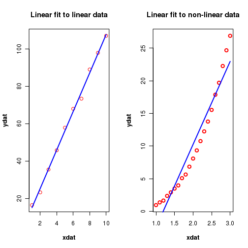
In the above figure, the plot on the left side depicts a stright line fitted to a data whose actual trend is fairly linear. On the other hand, the plot on the right side shows a best fit to a data that actually has a non-linear trend. But both are "best fit" to a stright line through data points.
Therefore, it is necessary to have a parameter that distinguishes between these two cases. A parameter that indicates the extend to which the data points are aligned to the fitted line. We should derive an expression for such a parameter from the data points \((x_i, y_i)\) and the values of fitted coefficients \( (b_0, b_1) \). Such a parameter is called "coefficient of determination" or the \(r^2~\) (r-square) parameter. We will now derive the parameter.
The coefficient of determination, $r^2$
To obtain a number that represents the quality of the fit, we compare the scateering of the data points about the fitted line with their scattering around their mean value $\overline{y}$
In the Figure-5 below, the blue line is the regression line through the data points that are represented by red circles.
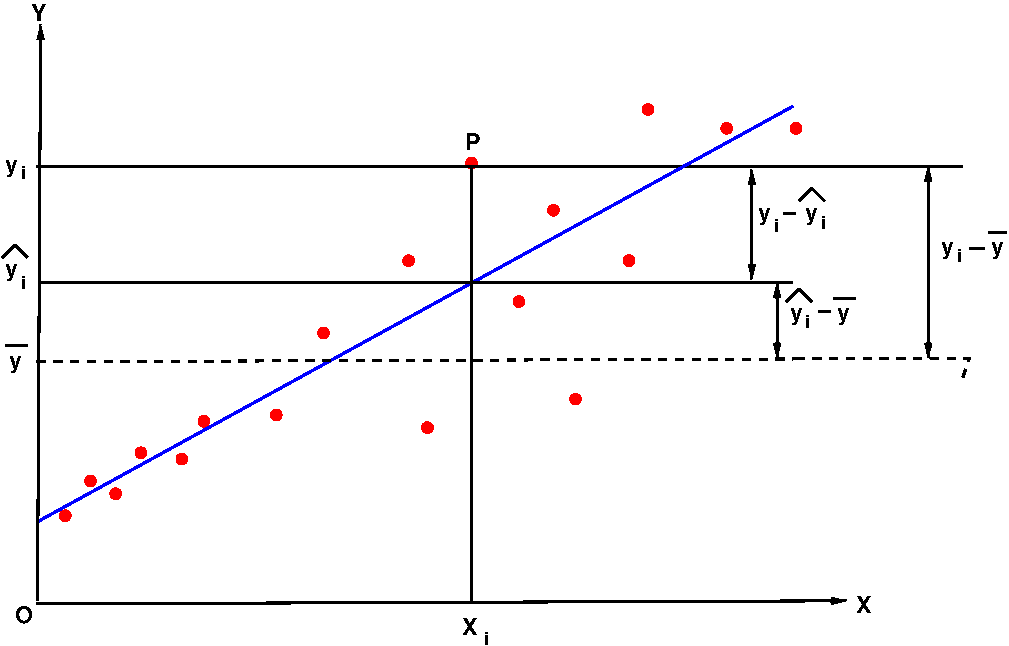
We consider the following quantities shown in the figure:
$x_i$ = the X value of the $i^{th}$ data point named P $y_i$ = the Y value of the $i^{th}$ data point named P $\hat{y_i} = y_i(x_i) = b_0 + b_1x_i = $ the value of fitted $Y$ for a given $x_i$ $\overline{y} = $ mean of all the $y_i$ values of the data set.
In the next step, we proceed to look at the deviations between the quantities $y_i$, $\overline{y}$ and $\hat{y_i}$ as follows:
$t_i = y_i - \overline{y}~~$ is the deviation of y-value of a data point i from the sample mean of all y values This deviation from the sample mean can be decomposed into two parts. We define, $m_i = \hat{y_i} - \overline{y}~~$ is the deviation of the fitted y-value of a data point i from the sample mean $\overline{y}$. $~~~~~~~~~~~~~~~~~~~~~~~~~~~~~~~~~~~~~$ this quantity is "explained by the model" $e_i = y_i - \hat{y_i}~~$ is the deviation of a $y_i$ from the corresponding fitted value. $~~~~~~~~~~~~~~~~~~~~~~~~~~~~~$ This is called the "residual associated with $y_i$". $~~~~~~~~~~~~~~~~~~~~~~~~~~~~~$ This can be thought of as a "deviation unexplained by the model" For every data point i,$~~~t_i = m_i ~+~e_i$ We will now consider the sum square of the above three deviations over all the data points. We define, $ SST~=~\displaystyle \sum_i t_i^2 =\displaystyle \sum_i (y_i - \overline{y})^2~~~$ is the amount of variation in the response variable y. $ SSR~=~\displaystyle \sum_i m_i^2 =\displaystyle \sum_i (\hat{y_i} - \overline{y})^2~~~$ is the variation in y explained by the regression model $ SSE~=~\displaystyle \sum_i e_i^2 =\displaystyle \sum_i (y_i - \hat{y_i})^2~~~$ variation of y left unexplained by the regression model The following relationship that exists between the above three variances is given below (proof skipped):As the data points get closer and closer to the best fit line, $~~r^2 \rightarrow 1$ As the data points deviate more and more form the best fit line, $~~r^2 \rightarrow 0$
$r^2$-value and correlation
The $r^2$ value of the fit is related to the Pearson's correlation coefficient $cor(X,Y)$ between the variable X and Y.
It can be shown that,
Thus, the r^2 value of the best fit $y = b_0 + b_1x$ is equal to the square of the Pearson correlation coefficient between x and y variables. We can get the $r^2$ value of the least square fit to stright line by computing the Pearson correlation coefficient between X and Y variables and squaring it, even before performing the fit.
Correlation between y and $\hat{y}$
We mention another important result by skipping the proof.
It can be shown that the correlation between the fitted value $\hat{y}$ and the response variable $y$ is same as the correlation between variable x and y:
Hypothesis testing regression coefficients
After estimating the linear regressioncoefficients $b_0$ and $b_1$ by using the method of least squares, we perform hypothesis tests to obtain their statistical significance.
Statistical test for the slope $\beta_1$We set up a statistical test for testing whether the slope $\beta_1$ of the population is equal to zero under the null hypothesis that there is no liear relationship between the independent variable x and the dependent variable y in the data. Accordingly, the statements of the null and alternate hypothesis are:
$~~~~~~~~~~~~~~~~~~~H_0 : \beta_1~=0~~~~~~~$ (The predictor variable X is not useful for making predictions) $~~~~~~~~~~~~~~~~~~~H_1 : \beta_1 \neq 0~~~~~$ (The predictor variable x is good for making predictions).
In general, the test statistic is a t-variable defined by,The intercept is the value of y when x is zero. On many occasions, the value x=0 for the data may not be meaningful. Still, we set up a procedure for performing the hypothesis testing for the intercept $\beta_0$.
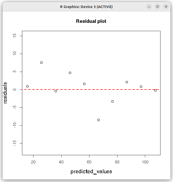
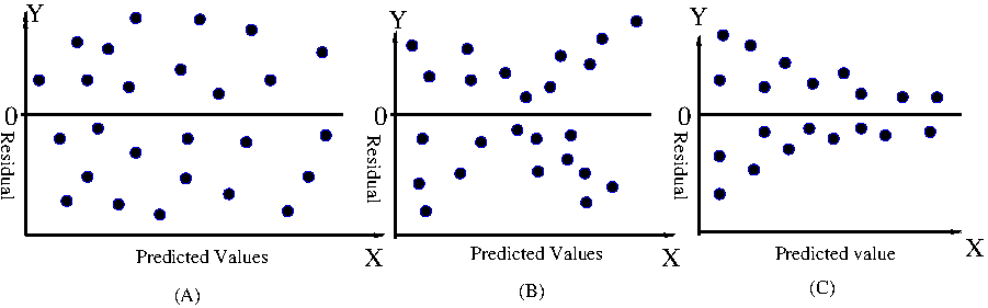
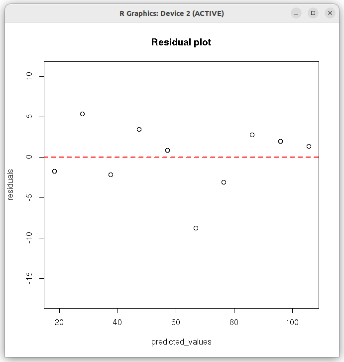
We define the null and alternate hypothesis for the test as, $~~~~~~~~~~~~H_0: \beta_0 = \beta$ $~~~~~~~~~~~~H_A: \beta_0 \neq \beta$ Under the null hypothesis, the tet statistics is defined using the fitted intercept $b_0$ following ususal procedure as, \(~~~~~~~~~~~~~~~t~=~\dfrac{b_0 - \beta}{SE(b_0)}~~~~~~\) has a t-distribution with (n-2) degrees of freedom. Here, $SE(b_0)$ is a standard error on the estimated coefficient $b_0$. Skipping the derivation, we repoduce here the expression for $SE(b_0)$ in terms of data variables as metioned in the genral literature: \(SE(b_0)~=~ \sqrt{\dfrac{\displaystyle \sum_i(y_i - \hat{y_i})^2}{n-2}} \displaystyle{\sqrt{\dfrac{1}{n}~+~\dfrac{\overline{x}^2}{\displaystyle \sum_i(x_i - \overline{x_i})^2}}} \) Under the null hypothesis, the test statistic is defined as,Inspecting the residuals in linear regression - The residual plot. In linear regression, for each daya point, the value $y_i$ of the data points deviates from the fitted value. At a give $x_i$, the difference between the fitted value $\hat{y}$ and the data value $y_i$ is called residual. Since $y_i$ values are assumed to be from a Gaussian distribution, if the fitting is perfect, then residuals $\epsilon_i = y_i - \hat{y}$ should fluctuate symmetrically around zero value. The residual plot is a scatter plot between the predicted values $\hat{y}$ and the corresponding residuals $\epsilon_i = y_i - \hat{y}$. In Figure-6 below, three types of scattering patterns in residual plots are depicted: In the ideal case, the variance of the dependent variable should be same over the entire range of the data. Therefore, we expect the residuals to be scattered unifirmly around the zero value across the entire range of predicted values, as shown in Figure-6(A) above. This property is called homoscedasticity. The regression method is base on the assumption that the data has homoscedasticity. In the scatter plots depicted in Figure-6(B) and Figure-6(c) above, we find a pattern in the residual plot across the range of fitted values. The residual values are not scattered uniformly around zero value across the predicted values. There is a trend in the scatter plot. Any pattern in the residual plot is called heteroscedasticity. The trend in the residual plot (heteroscedasticity) is likely an indication that the parameters used in our model have not best captured the relationship in the data. The residual plot carries this important information. Important assumptions of linear regression> 1. The observations are independent. 2. Linear relationship exists between the independent and dependent variables. 3. Nome of the predicted variables are correlated with each other (called "collinearity") 4. Homoscedasticity: The residuals have constant variance at every point in the linear model 5. The residuals are normally distributed.
Example Calculations for Linear regression
Hypothesis testing the entire model: the F-test To perform the F-test for the entire model, we need to compute the F statistic using the expression, \(~~~~~~~~~~~~~~~~~F~=~\dfrac{SSR/df_{SSR}}{SSE/df_{SSE}}~~~~\) We have, \( SSR~=~\displaystyle\sum_i(\hat{y_i} - \overline{y})^2~=240.0,~~~~~~~~~~df_{SSR}~=~2 \) \( SSE~=~\displaystyle\sum_i(y_i - \hat{y_i})^2~=0.84,~~~~~~df_{SSE}~=~n-p-1~=9-2-1~=~6 \) Substituting, we get F-statistic as, \(~~~~~~~F~=~\dfrac{(240/2)}{(0.84/6)}~=~857.14~~\) This is an F-distribution with $(p,n-p-1)$ degrees of freedom. The critical value to a significance level of $\alpha=0.05$ is, \(~~~~~~~~F_c~=~F_{1-\alpha}(p,n-p-1)~=F_{0.95}(2,6)~=~5.1\) Since $~~~F \gt F_c,~~$ we reject the null hypothesis $H_0:\beta_0=\beta_1=0$ to a significant level of 0.05. We conclude that the linear model we fitted shows a significant variation in the dependent variable when compared to the null model which assumes no variation. In fact, the F value of the test is so large that the corresponsing p-value is very very small.
Hypothesis testing the entire model: the F-test To perform the F-test for the entire model, we need to compute the F statistic using the expression, \(~~~~~~~~~~~~~~~~~F~=~\dfrac{SSR/df_{SSR}}{SSE/df_{SSE}}~~~~\) We have, \( SSR~=~~=1609.25,~~~~~~~~~~df_{SSR}~=~2 \) \( SSE~=~=22.432,~~~~~~df_{SSE}~=~n-p-1~=10-2-1~=~7 \) Substituting, we get F-statistic as, \(~~~~~~~F~=~\dfrac{(1609.25/2)}{(22.432/7)}~=~251.1 ~~\) This is an F-distribution with $(p,n-p-1)$ degrees of freedom. The critical value to a significance level of $\alpha=0.05$ is, \(~~~~~~~~F_c~=~F_{1-\alpha}(p,n-p-1)~=F_{0.95}(2,7)~=~4.74\) Since $~~~F \gt F_c,~~$ we reject the null hypothesis $H_0:\beta_0=\beta_1=0$ to a significant level of 0.05. We conclude that the linear model we fitted shows a significant variation in the dependent variable when compared to the null model which assumes no variation. In fact, the F value of the test is so large that the corresponsing p-value is very very small.
Linear Regression in R
For many additional parameters and their usage, typeIn R, the function lm() performs the linear regression of data between two vectors. It has the option for weighted and non-weighted fits, as well as nonlinear curve fitting. The function call with essential parameters is of the form,lm(formula, data, subset, weights) where,formula ------> is the formula used for the fit. For linear function, use "y~x"data --------> data frame with x and columns for datasubset ------> an optional vector specifying subset of data to be used.weights ------> an optionl vector with weights of fits to be used.
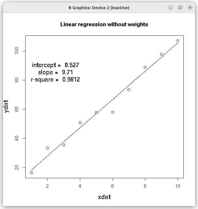
#  Linear regression in R

# lm is used to fit linear models

#-----------------------------------------------------------

##Straight line fit without errors

# define 2 data sets as vectors
xdat = c(1,2,3,4,5,6,7,8,9,10)
#ydat = c(16.5, 23.3, 35.5, 45.8, 57.9, 68.0, 73.4, 89.0, 97.9, 107.0)
ydat = c(16.5, 33.3, 35.5, 50.8, 57.9, 58.0, 73.4, 89.0, 97.9, 107.0)


# create a data frame of vectors
df = data.frame(x=xdat, y=ydat)


## function call for lm(). Here,x~y represents a linear relationship "y = a0 + a1 x "
#    (Use ydat~xdat-1 if you dont want intercept)

res = lm(ydat~xdat, df)  ## call the lm() function to perform linear model.

##Output results are stored in the list "res"
# In the above formuls, use y~x-1 if you don't want intercept


# Print the summary of entire analysis
print(summary(res))


# plot the results. First plot data points and then x versus fitted y)

plot(xdat,ydat, col="red", xlab="xdat", ylab="ydat", cex.lab=1.3, main="Linear regression without weights")
lines(xdat, res$fitted.values, col="blue")

## get slope, intercept and r-square vlues as strings.
inter_string = paste("intercept = ", round(res$coefficients[[1]], digits=3) )
slope_string = paste("slope = ", round(res$coefficients[[2]], digits=3) )
rsquare_string = paste("r-square = ", round(summary(res)$r.squared, digits=4))

## Write the above strings inside the plot.
## Forst plot normally, then decide the coordinates for the text centering in the graph
text(2.5,90,inter_string, cex=1.3)
text(2.5,85, slope_string, cex=1.3)
text(2.5,80, rsquare_string, cex=1.3)

X11()


## Create the residual plot

## predicted values
predicted_values = res$fitted.values

## residuals
residuals = (ydat - predicted_values)

## residual plot
plot(predicted_values, residuals, ylim=c(2.0*min(residuals), 2.0*max(residuals)), main="Residual plot" )
arrows( 0.5*min(predicted_values), 0, 1.5*max(predicted_values), 0, lty=2, col="red", lwd=2)


## Access the fitted reults as individual numbers.

## Uncomment the following line to see the residual plot, Q-Q plot, theoretical quantiles etc. (4 plots).
## These are plotted by the lm() function.
#plot(res)

# Uncomment the following line to print the interrcept
#print(paste("intercept = ", res$coefficients[1]))

# uncomment the following statement to print slope
#print(paste("slope = ", res$coeffcients[2])))

# uncomment the following statement to print the fitted values
# print(res$fitted.values)

# Uncomment the following statement to see 95% confidence interval
# confint(res, level=0.95)

# Uncomment the following line to print r-square value. Note that they are part of list "summary(res)"
# r.square = summary(res)$r.squared


##-----------------------------------------------------------------------------------
Running the above script in R prints the following output lines and graph on the screen:
In the above output, we gather that 1. The Intercept and slope have been estimated with an r-square value of 0.9812. 2. The p-value of the t-test for the slope is 0.0202 and corresponsing value for intercept t-test is $3.46 \times 10^{-8}$, indicating a very good estimate of these parameters. 3. The p-value of the F-test for the overall fit is $3.458 \times 10^{-8}$, indicating that the linear model fits the data very well. The following two figures are printed on the screen:Call: lm(formula = ydat ~ xdat, data = df) Residuals: Min 1Q Median 3Q Max -8.785 -2.051 1.101 2.593 5.354 Coefficients: Estimate Std. Error t value Pr(>|t|) (Intercept) 8.5267 2.9502 2.89 0.0202 * xdat 9.7097 0.4755 20.42 3.46e-08 *** --- Signif. codes: 0 ‘***’ 0.001 ‘**’ 0.01 ‘*’ 0.05 ‘.’ 0.1 ‘ ’ 1 Residual standard error: 4.319 on 8 degrees of freedom Multiple R-squared: 0.9812, Adjusted R-squared: 0.9788 F-statistic: 417 on 1 and 8 DF, p-value: 3.458e-08
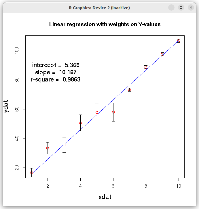
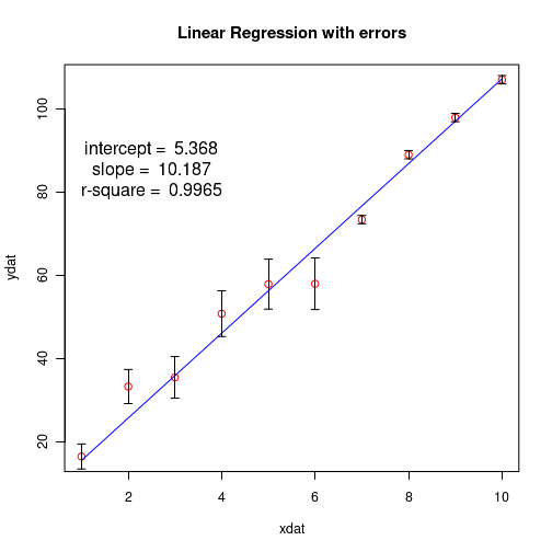
## Fit with errors (weights) on individual data points
## The weights are inverse of variances on data point.
## In our data, we call standard deviation as error.
## Hence the weights are inverse of square of errors.


xdat = c(1,2,3,4,5,6,7,8,9,10)
ydat = c(16.5, 33.3, 35.5, 50.8, 57.9, 58.0, 73.4, 89.0, 97.9, 107.0)
errors = c(3.0, 4.1, 5.0, 5.5, 6.0, 6.2, 1.0, 1.0, 1.0, 1.0)

df = data.frame(x = xdat, y=ydat, err=errors)

res = lm(y~x, data = df, weights = 1/(df$err)^2)

print(summary(res))


# plot the results

plot(xdat,ydat,col="red", main="Linear regression with weights on Y-values", cex.lab=1.3)
lines(xdat, res$fitted.values, col="blue")

## draw error bars on individual data points
## From each y-value, draw a vertical arrow connecting ydat-errors to ydat+errors and make arrow head 90 degree.
## This gives a vertical error bar.

arrows(xdat, ydat-errors, xdat, ydat+errors, length=0.05, angle=90, code=3)


## get slope, intercept and r-square vlues as strings.
inter_string = paste("intercept = ", round(res$coefficients[[1]], digits=3) )
slope_string = paste("slope = ", round(res$coefficients[[2]], digits=3) )
rsquare_string = paste("r-square = ", round(summary(res)$r.squared, digits=4))

## Write the above strings inside the plot.
## Forst plot normally, then decide the coordinates for the text centering in the graph
text(2.5,90,inter_string, cex=1.3)
text(2.5,85, slope_string, cex=1.3)
text(2.5,80, rsquare_string, cex=1.3)


X11()


## Create the residual plot

## predicted values
predicted_values = res$fitted.values

## residuals
residuals = (ydat - predicted_values)

## residual plot
plot(predicted_values, residuals, ylim=c(2.0*min(residuals), 2.0*max(residuals)), main="Residual plot", cex.lab=1.3 )
arrows( 0.5*min(predicted_values), 0, 1.5*max(predicted_values), 0, lty=2, col="red", lwd=2)


## Access the fitted reults as individual numbers.

## Uncomment the following line to see the residual plot, Q-Q plot, theoretical quantiles etc. (4 plots).
## These are plotted by the lm() function.
#plot(res)

# Uncomment the following line to print the interrcept
#print(paste("intercept = ", res$coefficients[1]))

# uncomment the following statement to print slope
#print(paste("slope = ", res$coeffcients[2])))

# uncomment the following statement to print the fitted values
# print(res$fitted.values)

# Uncomment the following statement to see 95% confidence interval
# confint(res, level=0.95)

# Uncomment the following line to print r-square value. Note that they are part of list "summary(res)"
# r.square = summary(res)$r.squared
Running the above script in R prints the following output lines and graph on the screen:
We conclude the following from the output of this weighted fit: 1. The computed slope pd 10.1866 is satistically significant (with small p-value of $9.71 \times 10^{-9}$, while the intercept value has a low statistical significance (p-value 0.167) in the t-test for coefficients. 2. The R-squared value of 0.9863 indicates a good weighted fit to the data points. 3. The extremely small p-value of $9.705\times 10^{-9}$ in the F-test shows the strength of overall linear model assumed for the data. 4. The fitted line is closer to the data points with smaller errors. The following two figures are printed on the screen:Call: lm(formula = y ~ x, data = df, weights = 1/(df$err)^2) Weighted Residuals: Min 1Q Median 3Q Max -3.2741 -0.1968 0.2908 0.8525 2.1393 Coefficients: Estimate Std. Error t value Pr(>|t|) (Intercept) 5.3680 3.5288 1.521 0.167 x 10.1866 0.4246 23.993 9.71e-09 *** --- Signif. codes: 0 ‘***’ 0.001 ‘**’ 0.01 ‘*’ 0.05 ‘.’ 0.1 ‘ ’ 1 Residual standard error: 1.668 on 8 degrees of freedom Multiple R-squared: 0.9863, Adjusted R-squared: 0.9846 F-statistic: 575.6 on 1 and 8 DF, p-value: 9.705e-09