CountBio
Mathematical tools for natural sciences
Statistics for Machine Learning
Multiple Linear Regression
In the linear regression, the relationship between a single explanatory variable x and a response variable y was modeled as
\(~~y~=~\beta_0~+~\beta_1 x\).
Suppose we have a situation where we have to model the relationship between a single response variable and more than one explanatory variables.
As an example, take a clinical trial that aims to study the weight of newborn infants on various health conditions of the mother. Suppose the
factors like mothers Body Mass Index, blood sugar, blood pressure, multiple pregnencies and complete blood count (all during pregnency) are supposed to
contribute to the infant's birth weight.
In this case, the body weight of the infant is the response variable that is assumed to be dependent on the five explanatory variables namely mother's
Body Mass Index, blood pressure, blood sugar, multiple pregnencies and the complete blood count. If we assume a linear relationship between the single
response variable and the five explanatory variable, we can model the system using the method of Multiple Linear Regression .
The Multiple Linear Regression models a linear relationship between multiple (ie., more than one) explanatory variables and a single response variable by performing a linear fit in a multidimensional space. Here, the explanatory variables are assumed to be independent of each other.
The linear relationship
Let us assume that our data has p explanatory (independent) variables and a single response (dependent) variable. We denote the response variable by the letter Y , and the p explanatory variables as $X_1$, $X_2$, $X_3$,.....,$X_p$ Since the explanatory variables are assumed to be independent, we can construct an orthogonal coocrdinate system of dimension (p+1) with one variable y and p explanatory variables. Though it is not possible to draw and visualize a coordinate system with more than 3-dimensions in this three dimensional world, mathematically it can exist in reality. Under this assumption, we perform a linear fit to the data between Y and X variables in this multidimensional orthogonal system. The linear relation is of the form, \(~~~~~~~~~~~~~~Y~=~\beta_0~+~\beta_1 X_1~+~\beta_2 X_2~+~\beta_3X_2~+~..........+~\beta_p X_p \)The symbolic representation of data
The data for multiple linear regression with one independent and p dependent variables consists of data points in (p+1) dimensions. Let there be n data points from our experiment or observations, denoted by $P_1$, $P_2$,.....,$P_n$. In terms of X and Y values, these data points can be represented as,The Leaset Square Regression
If the data consists of the entire population, we can write the linear model between the explanatory variables x and the response variable y for a general data point i as,The Least Square Regression in Matrix Notation
In the method of least square minimization with a single independent variable, the coefficients $b_0$ and $b_1$ were obtained by minimizing the residual with respect to these coefficients. This resulted in a set of two simultaneous equations with two vriables, which could be easily solved to get expressions for $b_0$ and $b_1$ in terms of data points $(x_i, y_i)$. In the case of least square minimization of multiple linear regression, there is a complication. A system with n data points and (p+1) coefficients will end up in n simulataneous equations with (p+1)unknown variables (coefficients b) to be determined. This system of many equations are very cumbersome to solve by elimination methods, which may end up with too many operations in higher dimensions. The n simultaneous equations with (p+1) variables can be elegantly solved if we write them down as matrix equations, and apply standard methods of linear algebra to solve them. Also, this matrix method has the great advantage of being seamlessly extended to non-linear relations between variables x and y. In the sections below, we will perform the least square minimization using matrix methods We start by writing a set of linear simultaneous equations for n data points and (p+1)variables using the notation given in eqn(1) above:$~~~~~~~~~~~(6)$ In the next step, we write down the set of above simultaneous equations (4) in matrix form:
The weighted Least Square Regression
The weighted data consists of weights $w_i$ for individual data points i. For example, weight $w_i$ may be the inverse of variance or any other error on $y_i$. With weighted data points, the sumsquare deviations are written as, \(~~~~~\chi^2~=~\displaystyle\sum_{i=1}^n e_i^2 ~ = ~ \displaystyle\sum_{i=1}^n w_i [~y_i~-~( b_0~+~b_1 x_{i1}~+~b_2 x_{i2}~+~b_3 x_{i3}~+~......+~b_p x_{ip})]^2 \) The minimization procedure for the above expression in matrix form leads to the following expression for the coeffficient matrix estimation:
Derivation of multiple linear regression coefficients
We have to minimize the sumsquare deviation ${\large\bf \overline{e}}^{T}{~\large\bf\overline{e}}$ with respect to the regression coefficients b. We proceed as follows:
The following two important properties of matrices is used in the derivation :
If ${\large\bf\overline{A}}$ and ${\large\bf\overline{A}}$ are tow matrices, then the following two properties hold good:
$({\large\bf\overline{A}} + {\large\bf\overline{B}})^{T}~=~{\large\bf\overline{A}}^{T}~+~{\large\bf\overline{B}}^{T} ~~~~~$ and $~~~~~~({\large\bf\overline{A}}~{\large\bf\overline{B}})^{T}~=~{\large\bf\overline{B}}^{T}~{\large\bf\overline{A}}^{T} $
Now we proceed with the minimizarion of ${\large\bf \overline{e}}^{T}{~\large\bf\overline{e}}$.
\( {\large\bf \overline{e}}^{T}{~\large\bf\overline{e}}~=~ ( {\large\bf\overline{Y}}~-~{\large\bf\overline{X}}~{\large\bf\overline{b}})^{T} (~{\large\bf\overline{Y}}~-~{\large\bf\overline{X}}~{\large\bf\overline{b}} ) \)
Expanding the Right Hand Side,
\( {\large\bf \overline{e}}^{T}{~\large\bf\overline{e}}~=~ {\displaystyle\left( {\large\bf\overline{Y}}^{T}~-~{\displaystyle\left( {\large\bf\overline{X}}~{\large\bf\overline{b}}\right)^{T} } \right)} ~ {\displaystyle\left( {\large\bf\overline{Y}}~-~{\displaystyle\left( {\large\bf\overline{X}}~{\large\bf\overline{b}}\right) } \right)} \)
\( {\large\bf \overline{e}}^{T}{~\large\bf\overline{e}}~=~ {\large\bf\overline{Y}}^{T}~{\large\bf\overline{Y}}~-~
\displaystyle\left({\large\bf\overline{X}}~{\large\bf\overline{b}}\right)^{T}~{\large\bf\overline{Y}}~-~ {\large\bf\overline{Y}}^{T}~\displaystyle\left({\large\bf\overline{X}}~{\large\bf\overline{b}}\right)~+~ {\displaystyle\left( {\large\bf\overline{X}}~{\large\bf\overline{b}}\right)^{T} }~{\displaystyle\left( {\large\bf\overline{X}}~{\large\bf\overline{b}}\right) } \)
Applying the two matrix properties mentioned in the beginning, we write
\( {\large\bf \overline{e}}^{T}{~\large\bf\overline{e}}~=~ {\large\bf\overline{Y}}^{T}~{\large\bf\overline{Y}} ~-~\displaystyle\left({\large\bf\overline{X}}~{\large\bf\overline{b}}\right)^{T}~{\large\bf\overline{Y}}~-~ \displaystyle\left({\large\bf\overline{X}}~{\large\bf\overline{b}}\right)^{T}~{\large\bf\overline{Y}}~-~{\displaystyle\left( {\large\bf\overline{X}}~{\large\bf\overline{b}}\right)^{T}} ~ {\displaystyle\left( {\large\bf\overline{X}}~{\large\bf\overline{b}}\right)} \)
\( {\large\bf \overline{e}}^{T}{~\large\bf\overline{e}}~=~ {\large\bf\overline{Y}}^{T}~{\large\bf\overline{Y}} ~-~{\large 2}\displaystyle\left({\large\bf\overline{X}}~{\large\bf\overline{b}}\right)^{T}~{\large\bf\overline{Y}}~-~{\displaystyle\left( {\large\bf\overline{X}}~{\large\bf\overline{b}}\right)^{T}} ~ {\displaystyle\left( {\large\bf\overline{X}}~{\large\bf\overline{b}}\right)} \)
\( {\large\bf \overline{e}}^{T}{~\large\bf\overline{e}}~=~ {\large\bf\overline{Y}}^{T}~{\large\bf\overline{Y}} ~-~{\large 2~}{\large\bf\overline{b}}^{T} {\large\bf\overline{X}}^{T}{~\large\bf\overline{Y}} ~+~ {\large\bf\overline{b}}^{T} {\large\bf\overline{X}}^{T} {\large\bf\overline{X}}~ {\large\bf\overline{b}}\)
$~~~~~~~~~~~~~~~~~~(D1)$
We will perform a least square minimization by minimizing ${\large\bf \overline{e}}^{T}{~\large\bf\overline{e}}$ with respect to the coefficients of the model which are the elements of $b$. For this, we have to take partial derivatives of the RHS of eqn(D1) with respect to elements of $b$, equate the resulting expressions to zero and solve for the coefficients.
Taking the partial derivatives of expression (D1) with respect to b and equating to zero, we write
\( \dfrac{\large \partial ({\large\bf \overline{e}}^{T}{~\large\bf\overline{e}}) }{\large \partial b}~=~\dfrac{\large \partial ({\large\bf\overline{Y}}^{T} {\large\bf\overline{Y}})}{\large \partial b} ~-~ {\large 2} \dfrac{\large\partial ({\large\bf\overline{b}}^{T} {\large\bf\overline{X}}^{T}{~\large\bf\overline{Y}} ) }{\large \partial b}~+~ \dfrac{\large\partial({\large\bf\overline{b}}^{T} {\large\bf\overline{X}}^{T} {\large\bf\overline{X}}~ {\large\bf\overline{b}})}{\large \partial b} ~=~{\large 0} \)
$~~~~~~~~~~~~~~(D2)$
The partial derivatives of the three matrices on the Right Hand Side of the equation (D2) are written here, skipping the proof:
\( \dfrac{\large \partial ({\large\bf\overline{Y}}^{T} {\large\bf\overline{Y}})}{\large \partial b} ~=~0 \)
\( \dfrac{\large\partial ({\large\bf\overline{b}}^{T} {\large\bf\overline{X}}^{T}{~\large\bf\overline{Y}} ) }{\large \partial b} ~=~ {\large\bf\overline{X}}^{T} {\large\bf\overline{Y}} \)
\( \dfrac{\large\partial({\large\bf\overline{b}}^{T} {\large\bf\overline{X}}^{T} {\large\bf\overline{X}}~ {\large\bf\overline{b}})}{\large \partial b} ~=~ {\large 2} \large{\large\bf\overline{X}}^{T} {\large\bf\overline{X}} {~\large\bf\overline{b}} \)
$~~~~~~~~~~~~~~(D3)$
\( {~~~\large\bf\overline{b}}~=~ \displaystyle \left( {\large\bf\overline{X}}^{T} {\large\bf\overline{X}} \right)^{-1} \large{\large\bf\overline{X}}^{T} {\large\bf Y} \)
$~~~~$ which is eqn(11) mentioned before.
Thus, for the linear regression model in matrix form given by ${\large\bf\overline Y}~~=~~{\large\bf\overline X} ~{\large\bf\overline b}~+~{\large\bf\overline e}$, the p coefficients of the fitted model can be obtained by the single column matrix ${\large\bf\overline{b}}$ of $(p+1)$ elements. The elements of ${\large\bf\overline b}$ are $(b_0, b_1, b_2, ..., b_p)$.
We skip the derivation of the regression coefficient expression for a weighted nonlinear
fit (equation(11-B)). This can be found in literature.
Important Note
Each of the The three expressions on the RHS of Equation D4 above, after proper multiplication of matrix elements, yield a single expression which are just functions of elements of appropriate matrices ${\large\bf\overline{y}}$, ${\large\bf\overline{X}}$ and ${\large\bf\overline{b}}$. Taking a partial derivative of these matrices with respect to b means, Just differentiate the expression with respect to each element of b, namely $b_0, b_1,b_2,....,b_p$ and write each one of these p derivative expression as elements of a single column matrix of dimension $p \times 1$. Then, this single column matrix of expressions in turn can be manipulated to give the above three results presented on the RHS of equation D3 above. Continuing our derivation, we plug in the expression for partial derivatived from D3 into D2 to get, \( {\large\bf \overline{e}}^{T}{~\large\bf\overline{e}}~=~ {\large -2}\displaystyle{\large\bf\overline{X}}^{T} {\large\bf\overline{Y}} ~+~ {\large 2} \large{\large\bf\overline{X}}^{T} {\large\bf\overline{X}} {~\large\bf\overline{b}}~=~{\large{0}} \) which gives, \( \displaystyle{\large\bf\overline{X}}^{T} {\large\bf\overline{Y}} ~=~ \large{\large\bf\overline{X}}^{T} {\large\bf\overline{X}} {~\large\bf\overline{b}} \) In order to recover the coefficient column matrix ${~\large\bf\overline{b}}$, we multiply both the sides of above matrix equation from the left by the term $ \displaystyle \left( {\large\bf\overline{X}}^{T} {\large\bf\overline{X}} \right)^{-1}$ to get \( \displaystyle \left( \large{\large\bf\overline{X}}^{T} {\large\bf\overline{X}} \right)^{-1} \large{\large\bf\overline{X}}^{T} {\large\bf\overline{X}} {~\large\bf\overline{b}} ~=~ \displaystyle \left( \large{\large\bf\overline{X}}^{T} {\large\bf\overline{X}} \right)^{-1}~\displaystyle{\large\bf\overline{X}}^{T} {\large\bf\overline{Y}} \) This results in and expression for the matrix ${~\large\bf\overline{b}}$ of the coefficients in terms of data matrixes ${~\large\bf\overline{X}}$ and ${~\large\bf\overline{Y}}$ as follows:The fitted values
The matrix of fitted values ${\large\hat {\large\bf\overline{Y}}}$ is obtained by multiplying ${\large\bf\overline{X}}$ and ${\large\bf\overline{b}}$ matrices.The Residuals
The residuals are given by,Computing the Sum Square values of the regression
The three important sum squares namely SST, SSR and SSE of linear regression can be computed from the ${\large\bf\overline{Y}}$, ${\large\hat {\large\bf\overline{Y}}}$ and the ${\large\bf\overline{H}}$ matrices. For this, we define the following two matrices to enable appropriate matrix operations: \begin{equation} {\large\bf\overline{D}}_{\large n \times n}~=~ \begin{bmatrix} 1 & 0 & 0 & 0 & ........& 0 \\ 0 & 1 & 0 & 0 & ........& 0 \\ 0 & 0 & 1 & 0 & ........& 0 \\ ...&...&...&...&..........& \\ ...&...&...&...&..........& \\ 0 & 0 & 0 & 0& ........& 1 \\ \end{bmatrix} \end{equation} The above diagonal matrix ${\large\bf\overline{D}}$ has n rows, n columns with all diagonal elements as 1 and off diagonal elements as zero. We define another square matrix of size $n \times n$ in which all the elements are 1: \begin{equation} {\large\bf\overline{J}}_{\large n \times n}~=~ \begin{bmatrix} 1 & 1 & 1 & 1 & ........& 1 \\ 1 & 1 & 1 & 1 & ........& 1 \\ 1 & 1 & 1 & 1 & ........& 1 \\ ...&...&...&...&..........& \\ ...&...&...&...&..........& \\ 1 & 1 & 1 & 1& ........& 1 \\ \end{bmatrix} \end{equation} Using the above two matrices and the hat matrix defined before, we can write down the expressions for the three sum squares in terms of matrix operations as,The r-square parameter and interpretation
Once we have determined the three sumsquare estimates, the $r^2$ value can be computed from sumsquare values using standard procedure:The Adjusted r-square value
As more and more predictor variables are inclued in the multiple linear regression, the value of $r^2$ parameter is artificially inflated. To avoid this, an adjusted r^2 value called $r_a^2$ is defined by normalizing the sumsquare values by their degrees of freedom:The Mean Square Error (MSE) and Standard Error (SE)
The Mean Square Error (MSE) and the Standard Error (SE) defined in equations (4) and (5) are written in terms of the fitted values and the original data as,Hypothesis testing of Multiple Linear Regression
Once the coefficients of the multiple linear regression are determined along with the sumsquare estimates, the next step in the analysis is to perform statistical tests on the overall validity of the model and the determined coefficients. Similar to the linear regression with a slope and intercept, the F-test and the t-test are performed:The F-test for the overall model
The F-test is the test for the overall significance of the fitted regression model. This test checks if a linear relationship exists between the response variables and at least one of the predictor variables. The null and the alternate hypothesis for the F-test for a regression with p coefficients are written as, $H_0:~\beta_1~=~\beta_2~=~........=~\beta_p~=0$ $H_A:~\beta_j \neq 0~~~$for at least one j value, where $j=1,2,3,....,p$ Following the ususal arguments of linear regression, under the null hypothesis, the F-statistics for the test is defined as,The t-test for the significance of estimated coefficients
The t-test computes the significance of the individual regression coefficients $\beta_1, \beta_2,....,\beta_p$ of the model. Addition of every significant variable to the model improves it, while the addition of every insignificant coefficient weakens the validity of the model. For every population coefficient $\beta_j$ in the model, we write the null and alternate hypothesis as, $~~~~~~~~~~~~H_0:~\beta_j = 0$ $~~~~~~~~~~~~H_A:~\beta_j \neq 0$ Let $s^2$ be the mean square estimate (MSE) of the model, as given by equation (19) above. We compute the covariance matrix defined by,Example Calculation for Multiple Linear regression
As an example problem, we consider the following simulated data set that was created by assuming a linear relationship between an independent variable Y and three dependent variables X1, X2 and X3:
$~~~~~~~~~~~~~~~~~~~~~~~~~~~~~~~~~~~~~~~~~~~~~~~~~~~~~~~~~~~~~~~~~~~~$ Table-1
\[
\begin{array}{|c|c|c|c|}
\hline
\text{Y} & \text{X1} & \text{X2} &\text{X3} \\
\hline
388.01 & 8.93 & 58.15 & 132.58 \\
389.79 & 10.63 & 53.07 & 104.34 \\
481.61 & 9.37 & 78.62 & 144.18 \\
445.86 & 10.75 & 68.3 & 131.86 \\
339.51 & 6.02 & 65.78 & 90.77 \\
295.26 & 2.83 & 55.59 & 95.7 \\
311.19 & 4.58 & 67.94 & 74.82 \\
289.74 & 6.6 & 61.76 & 73.48 \\
331.1 & 9 & 49.06 & 74.4 \\
390.09 & 11.89 & 59.38 & 120.04 \\
378.27 & 1.38 & 71.72& 147.16 \\
247.52 & 2.68 & 40.24 & 136.18 \\
300.83 & 9.09 & 47.51 & 95.2 \\
309.78 & 1.01 & 67.27& 87.04 \\
346.51 & 5.3 & 54.8 & 128.6 \\
346.39 & 6.09& 54.47& 109.94 \\
354.77 & 5.27 & 74.75 & 128.38 \\
354.76 & 5.43 &76.17 &76.43 \\
328.68 & 2.97& 64.7 &104.84 \\
304.97 & 11.47 &45.36 &88.93 \\
\hline
\end{array}
\]
We will now perform the regression analysis step by step. For matrix operations, we will use R package.
The entire script for these steps is given in the script section below. Also given is the R scrip for performing Multiple Linear Regression in R using lm() function.
For the above data table, the matrices ${\large\bf\overline{Y}}$ and ${\large\bf\overline{X}}$ are accordingly defined as,
\begin{equation}
{\large\bf\overline Y}~=~
\begin{bmatrix}
388.01 \\
389.79 \\
481.61 \\
445.86 \\
339.51 \\
295.26 \\
311.19 \\
289.74 \\
331.1 \\
390.09 \\
378.27 \\
247.52 \\
300.83\\
309.78 \\
346.51 \\
346.39 \\
354.77 \\
354.76 \\
328.68 \\
304.97 \\
\end{bmatrix}
{~~~~~~~~~~~~~~\large\bf\overline X}~=~
\begin{bmatrix}
1 &8.93 & 58.15 & 132.58 \\
1 & 10.63 & 53.07 & 104.34 \\
1 & 9.37 & 78.62 & 144.18 \\
1 & 10.75 & 68.3 & 131.86 \\
1 & 6.02 & 65.78 & 90.77 \\
1 & 2.83 & 55.59 & 95.7 \\
1 & 4.58 & 67.94 & 74.82 \\
1 & 6.6 & 61.76 & 73.48 \\
1 & 9 & 49.06 & 74.4 \\
1 & 11.89 & 59.38 & 120.04 \\
1 & 1.38 & 71.72& 147.16 \\
1 & 2.68 & 40.24 & 136.18 \\
1 & 9.09 & 47.51 & 95.2 \\
1 & 1.01 & 67.27& 87.04 \\
1 & 5.3 & 54.8 & 128.6 \\
1 & 6.09& 54.47& 109.94 \\
1 & 5.27 & 74.75 & 128.38 \\
1 & 5.43 &76.17 &76.43 \\
1 & 2.97& 64.7 &104.84 \\
1 & 11.47 &45.36 &88.93 \\
\end{bmatrix}
\end{equation}
All the matrix operations that will follow were done in R package. (see the code below which does these steps)
In this section, Multiple Linear Regression analysis for the data in Table-1 is performed with two R scripts. In the first one,
step by step analysis is carried out using basic Matrix operations in R. This gives us an insight into the steps involved in the analysis and enebales us to understand the nature of various quantities calculated in each step and print them. In the second script that follows, the Multiple Linear Regression is performed in R using lm() function of R stats library which was used before for linear regression.
Estimating coefficients
: \begin{equation} {~~~\large\bf\overline{b}}~=~ \displaystyle \left( {\large\bf\overline{X}}^{T} {\large\bf\overline{X}} \right)^{-1} \large{\large\bf\overline{X}}^{T} {\large\bf Y}~=~ \begin{bmatrix} -15.7285 \\ 9.7024 \\ 3.2245 \\ 0.9599 \end{bmatrix} \end{equation} This gives us, \( \bf {b_0=-15.7285~~, b_1 = 9.7024~~, b_2 = 3.2245~~ and ~~b_3 = 0.9599 }\)Estimating the fitted Y values
: The Hat Matrix is obtained as, \begin{equation} {\large\bf\overline{H}}~=~ {\large\bf\overline{X}} \displaystyle \left( {\large\bf\overline{X}}^{T} {\large\bf\overline{X}} \right)^{-1} \large{\large\bf\overline{X}}^{T} \end{equation} The above matrix is a square matrix of size 20. We do not print it here, since it is large. We estimate the fitted values by multiplying the Hat Matrix with $\large\bf\overline{Y}$ \begin{equation} {\large\hat {\large\bf\overline{Y}}}~=~{\large\bf\overline{H}}~ {\large\bf\overline{Y}~=~} \begin{bmatrix} 385.6768 \\ 358.6840 \\ 467.0858 \\ 435.3727 \\ 341.9141 \\ 282.8379 \\ 319.5978 \\ 317.9830 \\ 301.2006 \\ 406.3254 \\ 370.1751 \\ 270.7416 \\ 317.0409 \\ 294.5294 \\ 335.8348 \\ 324.5246 \\ 399.6614 \\ 355.9279 \\ 322.3446 \\ 327.1816 \\ \end{bmatrix} \end{equation}Estimating the residuals
: \begin{equation} {\large\bf\overline{e}}~=~{\large\bf\overline{Y}}~-~{\large\hat {\large\bf\overline{Y}}}~=~ \begin{bmatrix} 2.333198 \\ 31.106049 \\ 14.524216 \\ 10.487260 \\ -2.404095 \\ 12.422080 \\ -8.407830 \\ -28.243008 \\ 29.899381 \\ -16.235357 \\ 8.094945 \\ -23.221562 \\ -16.210932 \\ 15.250613 \\ 10.675173 \\ 21.865354 \\ -44.891408 \\ -1.167884 \\ 6.335414 \\ -22.211605 \end{bmatrix} \end{equation}Estimating the sumsquare values
: We have, $n = 20~~$, $p = 3$. We define a square matrix I of size 20 which has 1 along diagonals and non-diagonal elements zero. We also define a square matrix J of size 20 with all elements 1. \begin{equation} {\large\bf\overline I}_{\large 20 \times 20}=~ \begin{bmatrix} 1 & 0 & 0 & 0 & 0 & 0 & 0 & 0 & 0 & 0 & 0 & 0 & 0 & 0 & 0 & 0 & 0 & 0 & 0 & 0 \\ 0 & 1 & 0 & 0 & 0 & 0 & 0 & 0 & 0 & 0 & 0 & 0 & 0 & 0 & 0 & 0 & 0 & 0 & 0 & 0 \\ 0 & 0 & 1 & 0 & 0 & 0 & 0 & 0 & 0 & 0 & 0 & 0 & 0 & 0 & 0 & 0 & 0 & 0 & 0 & 0 \\ 0 & 0 & 0 & 1 & 0 & 0 & 0 & 0 & 0 & 0 & 0 & 0 & 0 & 0 & 0 & 0 & 0 & 0 & 0 & 0 \\ . & . & . & . & . & . & . & . & . & . & . & . & . & . & . & . & . & . & . & . \\ . & . & . & . & . & . & . & . & . & . & . & . & . & . & . & . & . & . & . & . \\ . & . & . & . & . & . & . & . & . & . & . & . & . & . & . & . & . & . & . & . \\ 0 & 0 & 0 & 1 & 0 & 0 & 0 & 0 & 0 & 0 & 0 & 0 & 0 & 0 & 0 & 0 & 0 & 0 & 0 & 1 \\ 0 & 0 & 0 & 1 & 0 & 0 & 0 & 0 & 0 & 0 & 0 & 0 & 0 & 0 & 0 & 0 & 0 & 0 & 0 & 0 \\ \end{bmatrix} \end{equation} \begin{equation} {\large\bf\overline J}_{\large 20 \times 20}=~ \begin{bmatrix} 1 & 1 & 1 & 1 & 1 & 1 & 1 & 1 & 1 & 1 & 1 & 1 & 1 & 1 & 1 & 1 & 1 & 1 & 1 & 1 \\ 1 & 1 & 1 & 1 & 1 & 1 & 1 & 1 & 1 & 1 & 1 & 1 & 1 & 1 & 1 & 1 & 1 & 1 & 1 & 1 \\ 1 & 1 & 1 & 1 & 1 & 1 & 1 & 1 & 1 & 1 & 1 & 1 & 1 & 1 & 1 & 1 & 1 & 1 & 1 & 1 \\ 1 & 1 & 1 & 1 & 1 & 1 & 1 & 1 & 1 & 1 & 1 & 1 & 1 & 1 & 1 & 1 & 1 & 1 & 1 & 1 \\ . & . & . & . & . & . & . & . & . & . & . & . & . & . & . & . & . & . & . & . \\ . & . & . & . & . & . & . & . & . & . & . & . & . & . & . & . & . & . & . & . \\ . & . & . & . & . & . & . & . & . & . & . & . & . & . & . & . & . & . & . & . \\ 1 & 1 & 1 & 1 & 1 & 1 & 1 & 1 & 1 & 1 & 1 & 1 & 1 & 1 & 1 & 1 & 1 & 1 & 1 & 1 \\ 1 & 1 & 1 & 1 & 1 & 1 & 1 & 1 & 1 & 1 & 1 & 1 & 1 & 1 & 1 & 1 & 1 & 1 & 1 & 1 \\ \end{bmatrix} \end{equation} \begin{equation} SST~=~{\large\bf\overline{Y}}^T {\displaystyle \left[ {\large\bf\overline{D}}~-\left( \dfrac{1}{n} \right) {\large\bf\overline{J}} \right] {\large\bf\overline{Y}} }~=~57422.69 \end{equation} \begin{equation} SSR~=~{\large\bf\overline{Y}}^T {\displaystyle \left[ {\large\bf\overline{H}}~-\left( \dfrac{1}{n} \right) {\large\bf\overline{J}} \right] {\large\bf\overline{Y}} }~=~49700.43 \end{equation} \begin{equation} SSE~=~{\large\bf\overline{Y}}^T {\displaystyle \left[ {\large\bf\overline{D}}~-{\large\bf\overline{H}} \right] {\large\bf\overline{Y}} }~=~7722.26 \end{equation} We see that, within numerical errors, $~~SST~=~SSR~+~SSE$Estimating the r-square values
: $r^2~=~1 - (SSE/SST)~=~1-\dfrac{7722.26}{57422.69}~=~0.8655 $ ${\large r_a^2}~=~\displaystyle{ 1 - \dfrac{\left(\dfrac{SSE}{n-p-1}\right) }{\left(\dfrac{SST}{n-1}\right)}}~=~\displaystyle{ 1 - \dfrac{\left(\dfrac{7722.26}{20-3-1}\right) }{\left(\dfrac{57422.69}{20-1}\right)}}~=~ 0.8403$Estimating the Mean Square Error (MSE) and Residual Standard Error (SE)
: $MSE = S^2~ = \dfrac{SSE}{(n-p-1)}~=~\dfrac{7722.26}{(20-3-1)}~=~482.64$ $SE~=~\sqrt{MSE}~=~S~=~\sqrt{482.64}~=~21.97$Hypothesis testing overall model : The F-test
: $F~=~{\displaystyle {\dfrac{\left(\dfrac{SSR}{p}\right)}{\left(\dfrac{SSE}{n-p-1}\right)}}}~=~{\displaystyle {\dfrac{\left(\dfrac{49700.43}{3}\right)}{\left(\dfrac{7722.26}{20-3-1}\right)}}} ~=~34.33~~~~~~~~~~is~~F(p,n-p-1) $ p-value for the F-test in R = $3.35 \times 10^{-7}$Hypothesis testing the coefficients: The t-test
: Compute the Covariance matrix: \begin{equation} {\large\bf\overline{C}}~=~S^2 \displaystyle \left( {\large\bf\overline{X}}^{T} {\large\bf\overline{X}} \right)^{-1}~=~ \begin{bmatrix} 1397.503565 & -23.4228967 & -13.75803129 & -3.58118863 \\ -23.422897 & 2.2954208 & 0.16118637 & -0.01337670 \\ -13.758031 & 0.1611864 & 0.23444143 & -0.01434281 \\ -3.581189 & -0.0133767 & -0.01434281 & 0.04233420 \\ \end{bmatrix} \end{equation} The square root of the diagonal elements of the Covariance matrix give the Standard Errors (SE) of the 4 coefficients: \( {\large S_{b_0}} ~= \sqrt{1397.503}~=37.38 \) \( {\large S_{b_1}} ~= \sqrt{2.2954}~=1.515 \) \( {\large S_{b_2}} ~= \sqrt{0.2344}~=0.484 \) \( {\large S_{b_3}} ~= \sqrt{0.04233}~=0.2057 \) We compute the t-statistic for each coefficient as follows: \( T_0~=~\dfrac{b_0}{S_{b_0}}~=~ \dfrac{-15.7285}{37.383}~=~-0.4207 \) \( T_1~=~\dfrac{b_1}{S_{b_1}}~=~ \dfrac{9.7024}{1.515}~=~6.404 \) \( T_2~=~\dfrac{b_2}{S_{b_2}}~=~ \dfrac{3.2243}{0.48419}~=~6.659 \) \( T_3~=~\dfrac{b_3}{S_{b_3}}~=~ \dfrac{0.9599}{0.2057}~=~4.665 \) Each one of the abovr t-statistic follows a t-distribution with $n-p-1~=~20-3-1~=~16~~$egrees of freedom. When the one sample, two sided t-test is performed in R for each one of these coefficients, we get the following two sided p-values: $p\_value(b_0)~=~0.3398$ $p\_value(b_1)~=~4.3643 \times 10^{-6}$ $p\_value(b_2)~=~2.7427 \times 10^{-6}$ $p\_value(b_3)~=~1.2930 \times 10^{-4}$ We can reject the null hypothesis of F and t-tests to the desired level of $\alpha$. Also, using equation(23), the $(1-\alpha)100\%$ Confidence intervals for the individual coefficients can be computed. Multiple Linear Regression in R
In this section, Multiple Linear Regression analysis for the data in Table-1 is performed with two R scripts. In the first one,
step by step analysis is carried out using basic Matrix operations in R. This gives us an insight into the steps involved in the analysis and enebales us to understand the nature of various quantities calculated in each step and print them. In the second script that follows, the Multiple Linear Regression is performed in R using lm() function of R stats library which was used before for linear regression.
1. Multiple Linear regression in R with Matrix operations
In the script below, following Matrix operations in R language are used:

If A and B are tow matrices,

A %*% B  -->  performs matrix multiplication of matrices A and B.

t(A) --> returns the transpose matrix of A

solve(A) -->  returns the inverse of the matrix A

Every section of the script is commented. The steps are same as described in the model calculation

described above.


The simulated  data set shown in Table-1 before consists of three independent variables X1, X2, X3
 and one dependent variable Y.

We assume a linear relationship between Y and X.

The data from table-1 is stored in the simple text file  MLR_simulated_data.txt and the script
below reads it into a data frame:
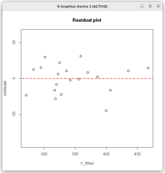
## R script on multiple linear regression with intermittent steps
## Uses matrix operations of R

## read data file -  simulated data
dat = read.table(file="MLR_simulated_data.txt", header=TRUE)

## Column matrix of dependent variable
Y = as.matrix(dat$Y) ## size 20x1

## Add a first clum with 1's to represent intercept in the data frame
Xf = data.frame( (rep(1,nrow(dat))), dat[, 2:4])

## Inlcude name of intercept in column names
names(Xf) = c("Inter", "X1","X2","X3")

## Data X matrix of independent variables
X = as.matrix(Xf)

##  Get the coefficient matrix b using matrix operations on X and Y

b = solve( (t(X) %*% X) ) %*% t(X) %*% Y   ## solve(M) gives the inverse of matrix M

b = round(b, digits=4)

## print coefficients
print("coefficients :")
print(b)
print("--------------------")

## Get the fitted values. But this gives just a avector of fitted values.
## Instead, use the Hat matrix below to get Y_fitted, which will be a column matrix
#  Y_fitted = (b[1] * X[,1]) + (b[2] * X[,2])  + (b[3] * X[,3]) + (b[4] * X[,4])
#  print(Y_fitted)


## Get the Hat Matrix H
H = X %*% solve( t(X) %*% X ) %*% t(X)

## using Hat matrix, get Fitted Values Y_fitted as a column matrix of size (20,1)
Y_fitted = H %*% Y

## Compute the residuals matrix - a column matrix of size(20,1)
e = Y - Y_fitted
# print(e)


## Estimating the sumsquare values

## number of data points
n = nrow(dat)

## number of coefficients
p = 3  ## ( apart from b0, three coefficients b1, b2, b3)

## Diagonal matrix I of size n
I = diag(1, n, n)

# A square matrix of size n with 1's
J = matrix(data=1, nrow = n, ncol = n)

## We  compute the three sumsquare values

SST = as.numeric(  t(Y) %*% (I - (1/n)*J) %*% Y )

SSR = as.numeric(  t(Y) %*% (H - (1/n)*J) %*% Y  )

SSE = as.numeric(  t(Y) %*% (I - H) %*% Y                            )
print("Sum Square Values :")
print(paste("SST = " ,SST))
print(paste("SSR = " ,SSR))
print(paste("SSE = " ,SSE))
print("-----------------------------------")


## Estimating the r-square value

r_square = 1 - (SSE/SST)

print(paste("r-square = ", round(r_square, digits=4)))

## Eatimaye the adjusted r-square

r_square_adjusted = 1 - ( (SSE/(n-p-1))/(SST/(n-1)) )

print(paste("adjusted_r-square = ", round(r_square_adjusted, digits=4)))

print("----------------------------------------")

## The Mean Square Error (MSE) of the model

MSE = SSE/(n-p-1)

MSE = round(MSE, digits=2)

print(paste("The Mean Square Error MSE = ", MSE))


## The Residual Standard Error (SE)

SE = sqrt(MSE)

print(paste("The residual standard error = ", round(SE, digits=3), " on ",n-p-1,

           " degrees of freedom"))

print("-------------------------------------------------")


## Hypothesis testing - The F-test

F = (SSR/p)/(SSE/(n-p-1))

F = round(F, digits=2)

p_value_F_test = format( 1 - pf(F, p, n-p-1), scientific=TRUE, digits = 3)

print(paste("F Statistic = ", F, "   degrees of freedom = ", p,",",n-p-1,"

            p-value = ", p_value_F_test))

print("-----------------------------------------------------")

tval = c()
pval = c()
SEvar = c()

## Hypothesis testing: The t-test for every coefficient in a for loop

C = MSE * solve(t(X) %*% X)

for(i in 1:length(b)) {

## sei is the square root of the corresponding diagonal element of C matrix.
##  It is the standard error on coefficient i

  sei = sqrt(C[i,i])

  Ti = b[i]/sei ## the t statistic for coefficient i

  if(Ti >= 0){
    pi = 1 - pt(Ti, n-p-1)
  }else{
    pi = pt(Ti, n-p-1)
  }

  tval = c(tval, Ti)
  pval = c(pval, pi)
  SEvar = c(SEvar, sei)
}

## convert p-value to two sided
p_value = pval*2

#print(p_value)


## print the results of t-test

varname = names(dat)  ## The first name is "Y". Change this to "Intercept"

varname[1] = "In"

tval = round(tval, digits=4)
SEvar = round(SEvar, digits=4)
p_value = format(p_value, format="r", digits=4)

print(paste("coefficients    ", "estimate     ", "Std.error     ", "t-value              ",

     "Pr(>t)"))
for(i in 1:length(b)){

 print(paste(varname[i], "           ", b[i],"          ",  SEvar[i], "      ", tval[i],

 "        ",   p_value[i]))

}


## Create the residual plot

## residuals
residuals = Y - Y_fitted

## residual plot
plot(Y_fitted, residuals, ylim=c(2.0*min(residuals), 2.0*max(residuals)), main="Residual plot" )
arrows( 0.5*min(Y_fitted), 0, 1.5*max(Y_fitted), 0, lty=2, col="red", lwd=2)


##---------------------------------------------------------------------------------------------
Running the above script in R prints the following output lines and graph on the screen:
The following Residual plot appears on the screen:[1] "coefficients :" [,1] Inter -15.7285 X1 9.7024 X2 3.2245 X3 0.9599 [1] "--------------------" [1] "Sum Square Values :" [1] "SST = 57422.6955199996" [1] "SSR = 49700.430294489" [1] "SSE = 7722.26522551094" [1] "-----------------------------------" [1] "r-square = 0.8655" [1] "adjusted_r-square = 0.8403" [1] "----------------------------------------" [1] "The Mean Square Error MSE = 482.64" [1] "The residual standard error = 21.969 on 16 degrees of freedom" [1] "-------------------------------------------------" [1] "F Statistic = 34.33 degrees of freedom = 3 , 16 p-value = 3.35e-07" [1] "-----------------------------------------------------" [1] "coefficients estimate Std.error t-value Pr(>t)" [1] "In -15.7285 37.3832 -0.4207 6.795e-01" [1] "X1 9.7024 1.5151 6.404 8.729e-06" [1] "X2 3.2245 0.4842 6.6596 5.485e-06" [1] "X3 0.9599 0.2058 4.6653 2.586e-04"
2. Multiple Linear Regression with lm() library function of R
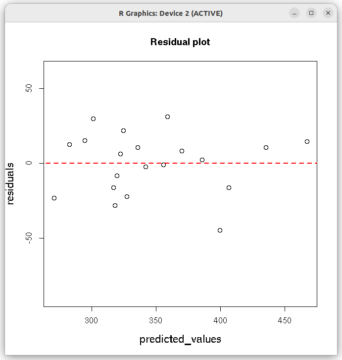
The Multiple Linear Regression analysis can be easily performed with the "lm()" function
of R stats library.


The steps are very similar to the one used in the ordinary linear regression in R.

In the R script below, we read the same data file "MLR_simulated_data.txt" with a dependent
variable Y and three independent variables X1, X2 and X3.

We will fit a linear model of the form Y = b0 + b1*X1 + b2*X2 + b3*X3

The steps are described in comments on each section of the R script given below.
Executing the above script in R prints the following output of results of the model on the screen:# R script for performing Multiple Linear Regression with lm() function of stats library ## Read the data table file as a data frame. dat = read.table(file="MLR_simulated_data.txt", skip=3, header=TRUE) # Perform multiple linear regression. Y is dependent variable, # other three (X1, X2, X3) are independent variables. ## This data is simulated. res = lm(Y ~ X1 + X2 + X3, data=dat) # print the summary. This has all information from the regression model print(summary(res)) ## Create the residual plot ## predicted values predicted_values = res$fitted.values ## residuals residuals = (dat$Y - predicted_values) ## residual plot plot(predicted_values, residuals, ylim=c(2.0*min(residuals), 2.0*max(residuals)), main="Residual plot", cex.lab=1.3 ) arrows( 0.5*min(predicted_values), 0, 1.5*max(predicted_values), 0, lty=2, col="red", lwd=2)
The following Residual plot appears on the screen:Call: lm(formula = Y ~ X1 + X2 + X3, data = dat) Residuals: Min 1Q Median 3Q Max -44.891 -16.217 4.334 12.948 31.106 Coefficients: Estimate Std. Error t value Pr(>|t|) (Intercept) -15.7285 37.3833 -0.421 0.679545 X1 9.7024 1.5151 6.404 8.73e-06 *** X2 3.2245 0.4842 6.660 5.49e-06 *** X3 0.9599 0.2058 4.665 0.000259 *** --- Signif. codes: 0 ‘***’ 0.001 ‘**’ 0.01 ‘*’ 0.05 ‘.’ 0.1 ‘ ’ 1 Residual standard error: 21.97 on 16 degrees of freedom Multiple R-squared: 0.8655, Adjusted R-squared: 0.8403 F-statistic: 34.33 on 3 and 16 DF, p-value: 3.351e-07