CountBio

Nonlinear Regression

The method of nonlinear regression models the nonlinear relationship between the independent(predictor) variable X and the dependent(response) variable Y.

We should first understand the two terms "linear relationship" and nonlinear relationship" between the predictor and response variables.

Suppose, a data consists of a response variable Y having a linear relationship with predictor variables $X_1$, $X_2$, $X_3$ and $X_4$. Using the method of multiple linear regression, we fit a linear relationship of the form,

$~~~~~~~~~~~~~~Y~=~\beta_0~+~\beta_1 X_1~+~\beta_2 X_2~+~\beta_3 X_3~+~\beta_4 X_4$

The genral form is,

$Y~=~(constant) + (parameter1 \times variable1) + (parameter2 \times variable2) +.... $


$~~~~(1)$




The model represented by eqn(1) above is a linear model since the predictor variable Y is expressed as a linear combination of paramters $\beta$ and response variables X.

Suppose we have a data in which the relationship between Y and X variables is modeled by a cubic polynomial function given by,

$~~~~~~~~~~~~Y~=~\beta_0~+~\beta_1 X_1~+~\beta_2 X_2^2~+~\beta_3 X_3^3 $
$~~~~~~~~~~~~~~~~~~(2)$



In the above equation(2), if we substitute the numeric values for the data points X, we end up with a relation in which Y is a linear combination of the model parameters $\beta$. Only the powers of variables X are tweeked to get a non-linear fit between Y and X variables. In this sense, the above model is actually linear in paramters $\beta$. We can fit this curve using multiple linear regression method we studied in the previous section, in which the variable $X1$, $X2$ and $X3$ are powered and Y is expressed as a linear combination with parameters $beta$ as in equation(1).

Though the mathematical relationship between Y and variables X are non-linear, the model is linear in parameters $\beta$ and the non-linear polynomial fit to the data is obtained through linear model by taking the powers of independent variables X.

In statistical analysis, a regression model is said to be linear when it is a linear function of paramters. The non linear fit is obtained by the linear combination of parameters and powers of the independent variables.

A regression model is nonlinear when the data is modeled by a function of one or more independent variables which is nonlinear in parameters.

As an example, the model represented by the exponential function$~~Y = \beta_1 \large{e}^{\small \beta_2 X} ~~$ is nonlinear beacause the independent variable Y cannot be written as a linear combinations of the parameters $\beta_1$, $\beta_2$ and the indepedent variable X

Examples for linear regression models(functions)

$~~~~~y~=~\beta_0~+~\beta_1 x ~~~~~~~~~~$ (simple linear relation )

$~~~~~y~=~\beta_0~+~\beta_1 x^2~+~\beta_2 x^2~+~\beta_3 x^3~~~~$ (cubic polynomial curve)

Examples for nonlinear regression models(functions)

$~~N(t) = \beta_1 \large{e}^{\small -\beta_2 t} ~~~~~~$ (Exponential decay curve in radioactivity)

$~~V(x)~=~\dfrac{\beta_1 x}{\beta_2 + x}~~~~~~~~$ (Michaelis Menton equation in enzyme kinetics)

$~~P(t)~=~\dfrac{\beta_1}{1~+~\beta_2 {\large e}^{-\beta_3 t}}~~~ $ (Logistic equation in population models)

From the above sets of equations, we note the following:

In linear regression, the values of the parameters $\beta$ are fixed. Any change in response variable Y is caused by change in the predictor variablex X.

The nonlinear regression is nonlinear in terms of the parameters $\beta$. Therefore, any change in the response variable Y is caused by the changes in the parameters $\beta$ as well as the predictor variables X.

$~~~~~~~~~~~~~~~~$

Nonlinear Least Square Regression method

Once the data set (X,Y) is given, we can fit a nonlinear model through the data points by the method of Leasr Square Regression, on the similar line as the linear regression. However, the minimization procedure with a nonlinear function is much more complicated than that we encountered in linear regression. It involves numerical methods.

In the sections below, a shorter form of the methodologies with essential steps is presented, skipping the details of the downstream algorithms. Many sophisticated algorithms have been developed for performing the nonlinear least square minimization. We will also learn a block level understanding of some of the important algorithms, without going into detailed steps.


Let the problem in hand has p coefficients $\beta_1$, $\beta_2$,$\beta_3$,.....,$\beta_p$ and m predictor variables denoted by $X_1$,$X_2$,$X_3$,....,$X_m$. Let Y be the response variable.

The nonlinear regression model is assumed to be of the form,

\begin{equation} \mu_i~=~f(\beta_1, \beta_2,....,\beta_p;~~x_{i1}, x_{i2}, x_{i3},.....,x_{im}) \end{equation}

$~~~~~~~~(1)$



where $\mu_i$ is the value of independent variable on the straight line representing the population data and $x_{ij}$ is the X-value of the data point i corresponding to the variable j. Here, f is the nonlinear function of parameters and variables which we want to fit to the data by least square minimization procedure.

For a data with n random samples, we write the nonlinear model as,

\begin{equation} y_i~=~f(b_1,b_2,b_3,....,b_p;~~x_{i1}, x_{i2}, x_{i3},.....,x_{im})~+~e_i \end{equation}

$~~~~~~~~(2)$



where $b_1,b_2,b_3,....,b_p$ are the best estimates of the corresponding $\beta$ parameters and $e_i$ is the error term for the data point i, as in the linear regression seen before.

Following the standard methods of regression theory, we write down the Residual Sum of Square (RSS) as,

\begin{equation} \displaystyle\sum_{i=1}^n e_i^2~=~\chi^2~=~\displaystyle\sum_{i=1}^n [y_i~-~f(b_1,b_2,b_3,....,b_p;~~x_{i1},x_{i2},x_{i3},....,x_{im}]^2 \end{equation}

$~~~~~~~~~(3)$





In order to get the best fit estimates $b_1$, $b_2$,....,$b_p$, we take the partial derivative of the $\chi^2$ function with respect to each parameter $b_j$ and equate the resulting expressions to zero. This gives us m simultaneous nonlinear equations on m parameters as variables. By solving these m nonlinear simultaneous equations, we can get the best fit parameter values $\beta_j$.

The resulting nonlinear simultaneous equations are given by,

\begin{equation} \dfrac{\partial \chi^2}{\partial b_1}~=~\dfrac{\partial}{\partial b_1} \displaystyle\sum_{i=1}^n [y_i~-~f(b_1,b_2,b_3,....,b_p;~~x_{i1},x_{i2},x_{i3},....,x_{im}]^2 \end{equation} \begin{equation} \dfrac{\partial \chi^2}{\partial b_2}~=~\dfrac{\partial}{\partial b_2} \displaystyle\sum_{i=1}^n [y_i~-~f(b_1,b_2,b_3,....,b_p;~~x_{i1},x_{i2},x_{i3},....,x_{im}]^2 \end{equation} ...... ........ ....... ........ ......... ...... ...... ...... ....... ........ \begin{equation} \dfrac{\partial \chi^2}{\partial b_m}~=~\dfrac{\partial}{\partial b_m} \displaystyle\sum_{i=1}^n [y_i~-~f(b_1,b_2,b_3,....,b_p;~~x_{i1},x_{i2},x_{i3},....,x_{im}]^2 \end{equation}






$~~~~~~~~~(4)$









The above simultaneous equations are nonlinear in coefficients $b_1,b_2,b_3,....,b_p$ and the independent variables $x_{i1},x_{i2},x_{i3},....,x_{im}$. They cannot be solved by the methods of matrix operations as we did in the case of multiple linear regression. (There the resuting simultaneous equations were linear in coefficients b). These nonlinear equations cannot be solved exactly to get the closed form of expressions for the parameters b in terms of data points (x,y) as we did in linear regression.

Hence we have to resort to numerical methods to solve these equations to get the coefficients of the models.

There are many numerical algorithms for performing nonlinear regression in multiparameters. Some of the important algorithms are: Gauss Newton algorithm, Levenberg-Marquardt algorithm, method of iteratively reweighted least squares etc. Many such algorithms exist in literature and implemented in various software tools and libraries for statistical analysis.

The foundational ideas behind the nonlinear least square minimization methods have been explained in the section titled Algorithms for nonlinear least square minimization.

Hypothesis testing regression coefficients

In linear regression theory, the standard error $SE(b_j)$ of an estimated parameter $b_j$ is an unbiased estimator of the corresponding population variance $\sigma_j$. Using this fact, a statistical t-test was constructed to test the hypothesis on the parameter $\beta_j$. These type of exact hypothesis test is mathematically possible in nonlinear regression theory. Hypothesis testing can be done only using approximate inference procedures.

For a nonlinear regression model, the Mean Squared Error (MSE) is computed using the Sum of Squared Error (SSE) from the data points $(x_i, y_i)$ and the regression function $f(b_1,b_2,...,b_p; .x_1,x_2,...,x_m)$ as, \begin{equation} Mean~Squared~Error~(MSE) ~~~~~S^2~=~{\displaystyle\dfrac{SSE}{n-p}} ~=~ \dfrac{\displaystyle\sum_{i=1}^n (y_i - f(\overline{b}, \overline{x}))^2}{n-p} \end{equation} The above MSE is not an unbiased estimator of the corresponding population varience $\sigma^2$. But the bias is small when the sample size is large.

The mathematical theory says that when the error terms $e_i$ are normally distributed and the sample size is large, the sampling distribution of the coefficients $\overline{b}$ is approximately normal.

In this case, an approximate varience of the regression coefficients are derived as,

$~~~~~~~~~~~\overline{s^2}~=~MSE \times (\overline{J}^T J)^{-1}$
$~~~~~~~~~~~~~~(5)$


where $\overline{J}$ is the Jacobian matrix of partial derivatives of f estimated at the final least square values of $\overline{b}$.

The computed parameters $\overline{b}$ of the model are unbiased estimates and are approximately normally distributed. $\overline{s^2}$ is called "the approximate estimate of the standard error".

An important fact is that this estimated standard error matrix $\overline{s^2}(\overline{b})$ is exactly in the same form as in the linear regression model.

Also, estimated variances of the parameters are at their minimum values, since the formula $\overline{s^2}~=~MSE \times (\overline{J}^T J)^{-1}$ estimates the minimum variance.

Based on these facts, we can carry out the statistical inferences for nonlinear regression in the same way as we do for the linear regression.

Statistical test

For a given parameter $b_j$ of the model, we can get the estimated standard deviation $s(b_j)$ using the variance matrix given by the equation(5) above.

Based on this, an approximate $(1-\alpha)100\%$ confidence interval for $\beta_j$ can be defined as,

$~~~~~~~CI~=~b_j \pm {\large t}_{1-\frac{\alpha}{2}, n-p}~s(b_j) $
$~~~~~~~~~~~~~~(6)$


where ${\large t}_{1-\frac{\alpha}{2}, n-p}$ is the $(1-\alpha)100$ percentile of the t distribution with (n-p) degrees of freedom.

An approximate one sided statistical t-test can be performed on the null hypothesis $~H_0: b_j=b_0$ to the significance level of $\alpha$ by defeining a t statistic:

$t_c~=~\dfrac{b_j - b_0}{s(b_j)}$
$~~~~~~~~~~~~~~~~(7)$




Reject null if $|t_c| \gt {\large t}_{1-\frac{\alpha}{2}, n-p}$

Validity of the large sample assumption

Ideally, if the sample size is large enough, the large sample assumtion made in the estimation of approximate quantities is valid. How do we know that the given sample size in our data is large enough so that we are safe to use large sample assumption?

One indication is the quick convergence of the procedure during the iterative estimation of coefficients. The quick convergence indicates that the linear approximation to nonlinear model is a good approximation and hence the asymptotic properties of regression estimates are good enough. Many other procedures mentioned in the literature to check the validity of this assumption.

See the following reference (an e-book):

http://www.cnachtsheim-text.csom.umn.edu/kut86916_ch13.pdf

Some Popular nonlinear models in Life Sciences

Quardratic Polynomial

$~~~~~~Y~=~b_0+b_1X+b_2X^2~~~~~~~~~~~~~$ Example: Hardy-Weinburg equation

Exponential function

$~~~~~~Y~=~a e^{bX}~~~~~~~~~~~~~~~$ Example: Exponential population growth

$~~~~~~Y~=~a e^{-bX}~~~~~~~~~~~~~~~$ Example: Radioactive decay, light absorption

Power law

$Y~=~a X^{b}~~~~~~~~~~~~~~$ Example: Metabolic scaling theory, biomass production, cell division

Logarithmic

$Y~=~a~+~b~log(X)~~~~~~~~~~~~~$ Example: logarithmic phase of bacterial growth

Rectangular Hyperbola

$Y~=~\dfrac{ax}{b+x}~~~~~~~~~~~~~$ Example: Michaelis-Menten equation in enzyme kinetics

Logistic Function

$Y~=~\dfrac{L}{1 + e^{-k(x-x_0)}}~~~~~~~~~~~~$ Example: Population growth, tumor growth, autocatalytic $~~~~~~~~~~~~~~~~~~~~~~~~~~~~~~~~~~~~~~~~~~~~~~~~~~~~~~~~~~~~~~~$ reactions in enzyme kinetics

Log-Logistic Function

$y~=~\dfrac{d}{1~+~\large{e}^{b[log(X) - log(c)]}}~~~~~~~~$Example: Dose and time response curves of drugs

Gaussian function

$y~=~a \large{e}^{-b~x^2}~~~~~~~$ Example: Probability density distributio of continuous variables


The general shape of these functions are plotted in Figure-1 below:

Nonlinear Regression in R

R has many library functions to perform nonlinear regression. The following three functions from stats library are prominently used:

1. $~~~~$ lm() function can fit the linear model, nonlinear models and oneway ANOVA. It uses an algorithm that solves least squares with QR decomposition method
"lm" stands for "Linear Model"

2.$~~~~$ nls() function performs nonlinear regression. It has three choices for the algorithm to be used. The default is "Gauss-Newton algorithm". The other two being "Golub-Pereyra algorithm for partially linear least-squares models" and the ‘nl2sol’ algorithm from the Port library.
"nls" stands for "Nonlinear Least Squares".

3.$~~~~$ glm() function can perform generalized linear models. The family of generalized linear models include logistic regression, Poisson regression and survival analysis. We can also use glm() function for linear and nonlinear regressions. The algorithm used is the "iteratively reweighted least squares", which is a second derivative method similar to Gauss-Newton method.
"glm" stands for "Generalised Linear Models"

In the following sections, we will fit different linear models using the three libraries.

Example-1 : Exponential fit with lm() function

The exponential function can be converted to a linear function through log transformation. We obtain the coefficients of exponential function from the coefficients of this linear fit.

Let the exponential function to be fitted be of the form,

$~~~~~~~~~~~~~~y~=~b_1~{\large e}^{b_2 x}$

Taking natural logarithm of both the sides, we get

$~~~~~~~~~~~~~~log(y)~=~log(b_1)~+~b_2 x$

Denoting $ y_l~=~log(y), ~~~c = log(b_1)$, we write above expression as,

$~~~~~~y_l~=~c~+~b_2 x~~~~~~~~~~~~$(Equation of a stringht line)

We now fit $y_l~=~log(y)$ versus x using the $lm()$ funciton in R to get the slope $b_2$ and the intercept c.

From this, we can recover the original coefficients of exponential fit as,

$~~~~~~~~~~b_1={\large e}^c~~~~and~~~~~b_2 = b_2$.


The lm() function for performing linear regression is described in the linear regression section. We reproduce the description here:

In R, the function lm() performs the linear regression of data between two vectors. 

It has the option  for weighted and non-weighted fits, as well as nonlinear curve fitting.

The function call with essential parameters is of the form,

 lm(formula, data, subset, weights) 

where,
$
 formula  ------>  is the formula used for the fit. For linear function, use "y~x"

 $~~~~~~~~~~~~~~~~~~~~~~~~$ The intercept term is included by default in the formula format.

 $~~~~~~~~~~~~~~~~~~~~~~~~$ Use  "y ~ x-1"  or  "y ~ 0 + x"  to remove the intercept.

 data  -------->  data frame with x and columns for data

 subset  ------> an optional vector specifying subset of data to be used.

 weights  ------> an optionl vector with weights of fits to be used. 

                        Weights are inversly proportional to the variences.

For many additional parameters and their usage, type help(lm) in R.

The data table is stored in csv file exponential_data.csv. This table contains the data describing a linear relationshi between two variaables "xdat" and "ydat" with errors on "ydat".

The script below reads it into a data frame, performs linear regression between log(ydat) and xdat to get the coefficients of linear fit. These are transformed back to the coefficients of exponential fit:

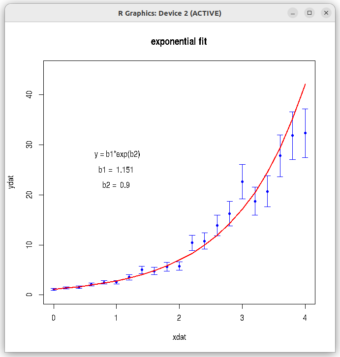
## fitting an exponential function to data

## fit of the form   y = b1*exp(b2 * x)

## taking log on both sides,    log(y) = log(b1) + b2*x

## so, we fit log(y)~x

## log(b1) is intercept. So, b1 = exp(intercept)

## b2 is the slope, as we get.

## then, y_fitted = b1*exp(b2*x)

## --------------------------------------------------



## read data file
dat = read.csv(file="./data_files/exponential_data.csv", header=TRUE)

xdat = dat$xdat

ydat = dat$ydat

err = dat$error

## error propagation while taking log of variable ydat.
err_log = err*(log(ydat)/ydat)

## Call the lm() function for linear fit between log(ydat) and xdat.
res = lm(log(ydat)~xdat, data = dat, weight = 1/err_log)

## print the summary of results
print(summary(res))

## retreive the slope and intercept
intercept = res$coefficients[[1]]
slope = res$coefficients[[2]]

## Get back the coefficient b1 of exponential fit.
b1 = exp(intercept)

b2 = slope

# Fitted y values
y_fitted = b1*exp(b2*xdat)


## Plot the data points with errors and fitted curve.
plot(xdat, ydat, col="blue", pch=20, main="exponential fit", ylim=c(0,45))
arrows(xdat, ydat+err, xdat, ydat-err, angle=90, code=3, length=0.06, col="blue")
lines(xdat, y_fitted, type="l", lw=2, col="red")
b1_string = paste("b1 = ", round(b1, digits=3) )
b2_string = paste("b2 = ", round(b2, digits=3) )
text(1,28, " y = b1*exp(b2)")
text(1,25,b1_string )
text(1,22, b2_string) 

Running the above script in R prints the following output lines and graph on the screen:

Call:
lm(formula = log(ydat) ~ xdat, data = dat, weights = 1/err_log)

Weighted Residuals:
     Min       1Q   Median       3Q      Max 
-0.36534 -0.13895 -0.03797  0.19807  0.42882 

Coefficients:
            Estimate Std. Error t value Pr(>|t|)    
(Intercept)  0.14106    0.02614   5.396 3.31e-05 ***
xdat         0.89983    0.01912  47.061  < 2e-16 ***
---
Signif. codes:  0 ‘***’ 0.001 ‘**’ 0.01 ‘*’ 0.05 ‘.’ 0.1 ‘ ’ 1

Residual standard error: 0.2565 on 19 degrees of freedom
Multiple R-squared:  0.9915,	Adjusted R-squared:  0.991 
F-statistic:  2215 on 1 and 19 DF,  p-value:  < 2.2e-16

In the above output, we gather that

1. The slope = 0.899 and the intercept $c=0.14106$.
From this, $b_1 = e^c = e^{0.14106}~=~1.1515$ and $b_2 = 0.899$.

Therefore, the fitted curve is $y = b_1 e^{b_2}~=~1.1515 \large{e}^{0.899}$

2. The adjusted $r^2$ value is 0.991, indicating a very good exponential fit to the data.

3. The significance tests (t-tests) for intercept and slope have yielded very small p-values, indicating a good statistical significance.

The plot created by the script with original data points and the fitted curve is shown below:

Example-2 : Polynomial fit with lm() function

In polynomial fit, the data is fitted with a polynomial function of degree n of the form,

$~~~~~~~~~~y(x)~=~b_0 + b_1 x + b_2 x^2 + b_3 x^3 + ........+ b_n x^n$

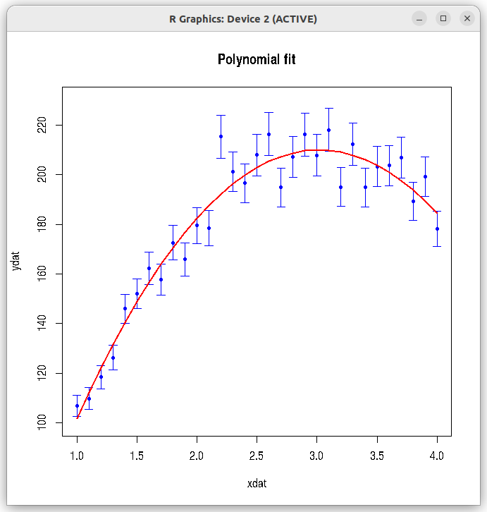
In this example, we fit a (quardratic) polynomial of degree 2 using the lm() function of R statistics library. The lm() can be called for polynomial fot in two formats:

1. By directly giving the orders of polynomials using I() function in the "formula" parameter:

$~~~~~~~~~~~~~~~~~~~~~~~~~$ mod <- lm(formula = ydat ~ I(xdat^2) + I(xdat^3), weights=1/error)

In the above function call, "formula = ydat ~ I(xdat^2) + I(xdat^3)" implies a polynomial formula $ y = b_0 + b_1 x^2 + b_2 x^3$ with explicit intercept term.

Use "formula = ydat ~ 0 + I(xdat^2) + I(xdat^3)" to remove the intercept from the fit.


2. By using the function poly() to input the polynomial function form to lm() :

mod <- lm(ydat ~ poly(xdat, 2, raw=2), data = dat, weights=1/error)

In the function call poly(xdat, 2, raw=2), the number "2" indicates a second order (quardratic) polynomial and the parameter call "raw=2" returns the coefficients of normal linear regression we presented in this tutorial. If this paramter "raw=2" is omitted, then, by default, orthogonal polynomials are returned. Use "raw=2" always.

The data table is stored in csv file polynomial_data.csv. This table contains the data describing a polynomial relationshi between two variaables "xdat" and "ydat" with errors on "ydat". The script below reads it into a data frame, performs polynomial regression between the variables ydat and xdat to get the coefficients of polynomial fit. We fit a quardratic polynomial of degree 2 for this data:

## fittng a data to polynomial

dat = read.csv(file="./data_files/polynomial_data.csv", header=TRUE)

xdat = dat$xdat

ydat = dat$ydat

error = dat$err

## If you remove raw=2, returns coefficients of orthogonal polynomial fit (dont use it).
## Use with raw=2, so that normal fitting values of coefficients are returned.

 mod <- lm(ydat ~ poly(xdat, 2, raw=2), data = dat, weights=1/error)



## Returns normal poplynomial fit coefficients b0, b1, b2 and b3.
## mod <- lm(formula = ydat ~ xdat + I(xdat^2) + I(xdat^3), weights=1/error)

## Fitted without first order xdat term. 
## Computes coefficients b0, b2 and b3, omitting b1.
## Looks better than second degree polynomial with xdat term shown above.
## mod <- lm(formula = ydat ~ I(xdat^2) + I(xdat^3), weights=1/error)


print(summary(mod))

y_fitted = mod$fitted.values


plot(xdat, ydat, col="blue", pch=20, main="Polynomial fit", ylim=c(100,230) )
arrows(xdat, ydat+error, xdat, ydat-error, angle=90, code=3, length=0.06, col="blue")
lines(xdat, y_fitted, type="l", lw=2, col="red")

Running the above script in R prints the following output lines and graph on the screen:

Call:
lm(formula = ydat ~ poly(xdat, 2, raw = 2), data = dat, weights = 1/error)

Weighted Residuals:
    Min      1Q  Median      3Q     Max 
-5.0216 -2.0250 -0.1788  2.2386  7.8692 

Coefficients:
                        Estimate Std. Error t value Pr(>|t|)    
(Intercept)              -31.811     10.681  -2.978  0.00593 ** 
poly(xdat, 2, raw = 2)1  160.231      9.695  16.527 5.64e-16 ***
poly(xdat, 2, raw = 2)2  -26.549      1.960 -13.544 8.15e-14 ***
---
Signif. codes:  0 ‘***’ 0.001 ‘**’ 0.01 ‘*’ 0.05 ‘.’ 0.1 ‘ ’ 1

Residual standard error: 3.031 on 28 degrees of freedom
Multiple R-squared:  0.9539,	Adjusted R-squared:  0.9506 
F-statistic: 289.7 on 2 and 28 DF,  p-value: < 2.2e-16

We can see that the adjusted R-square for the fit is 0.9506, indicating that it is a good fit to the data. Similarly, the results of t-test and F-test for the fit are also giving extremly low p-values.

The best fit curve is of the form,

$~~~~~~~y(x)~=~-32.811~+~160.231~x~-~26.549~x^2$

The plot created by the script with original data points and the fitted curve is shown below:

Example-3 : Nonlinear fit with nls() function

We will fit the Michaelis-Menton data of enzyme kinetics using nls() function of R stats library.

The function is of the form,

$~~~~~~~~~~~~~~y(x)~=~\dfrac{b_1 x}{b_2 + x} $

The function call with some of the essential parameters is of the form,




 nls(formula, data, start, algorithm, weights, ....) 





where,



 formula  ----------> is the relation between y and x that we want to fit.



 data  ------------> is the data frame with x,y and error(if used) for each data point.



 algorithm ---------> name of algorithm in string form. Three choices are there.

                         Gauss-Newton algorithm by default,  "plinear" for Golub-Pereyra

                         algorithm for partially linear least-squares models and

			 "port"’ for the ‘nl2sol’ algorithm from the Port lib

 weights  ------------> vector of weights, which is inverse of varience for each data point.

 start  -------------> a vector of initial values for the parameters.



(see manual for other parameters)

The R script presented below reads the data file "MM_kinetics_data.csv" and performs a nonlinear fit of MM kinetics form to the data.

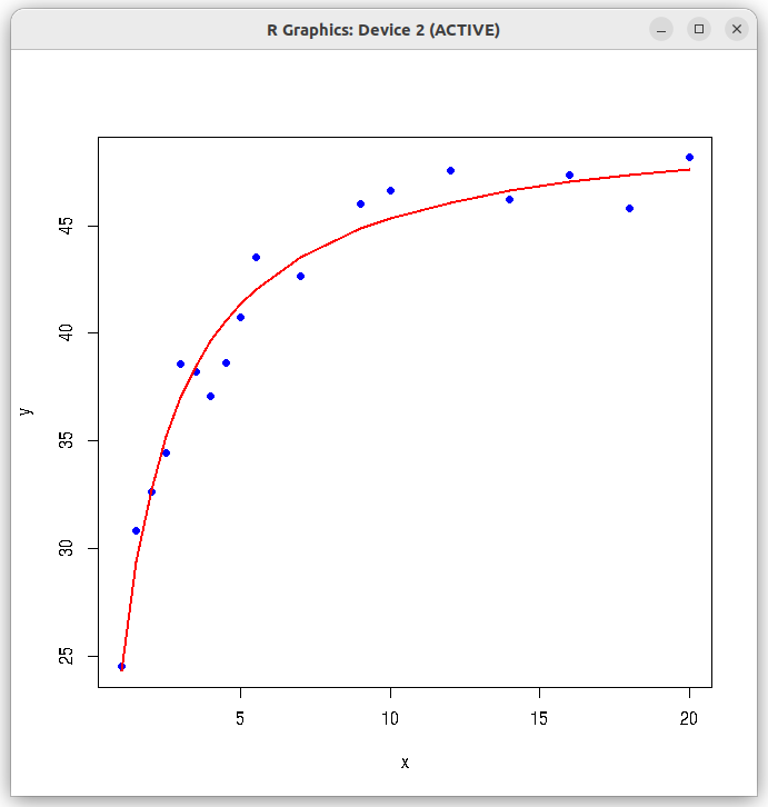
## Fitting MM kinetics (nonlinear) curve using nls function.

# Read the data file into data frame
dat = read.csv(file="./data_files/MM_kinetics_data.csv", header=TRUE)

## Extract x and y data vectors
y = dat$y

x = dat$x

## Call the nls function with MM kinetics formula
res <- nls(y ~ (b1 * x) / (b2 + x), start=list(b1=35, b2=2.0))

## Print the summary of results
print(summary(res))

## Plot datav points and the fitted curve.
plot(x,y,col="blue", pch=20, cex=1.3)
lines(x, predict(res), type="l", lwd=2, col="red")

Running the above script in R prints the following output lines and graph on the screen:

Formula: y ~ (b1 * x)/(b2 + x)

Parameters:
   Estimate Std. Error t value Pr(>|t|)    
b1 50.15639    0.66250   75.71  < 2e-16 ***
b2  1.06121    0.07473   14.20 1.73e-10 ***
---
Signif. codes:  0 ‘***’ 0.001 ‘**’ 0.01 ‘*’ 0.05 ‘.’ 0.1 ‘ ’ 1

Residual standard error: 1.294 on 16 degrees of freedom

Number of iterations to convergence: 6 
Achieved convergence tolerance: 1.971e-06