CountBio

Binary Logistic Regression

In the linear regression model, it is assumed that the dependent(response) variable y is quantitative, ie., the dependent variable y is a continuous function of the independent (predictive) variable x. It is also assumed that at each value of x, the corresponding value of y is normally distributed.

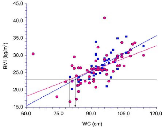
As an example, consider the scatter plot below modeling a linear relation between the Body Mass Index (BMI) and the weist circumference of adult women in a population:



(Plot taken from reference:
"The best criteria to diagnose metabolic syndrome in hypertensive Thai patients"
$~~~~~~~~~~~~~$Panita Limpawattana et.al.,
Journal of the Medical Association of Thailand, 91(4):485-90, April 2008 )

In the above data, the Body Mass Index (BMI) and the Weist Circumferece both are continuous variables with values represented by real numbers. The lines are linear fit to the blue and red data points.

Data with two (binary) or more discrete outcomes

On many occasions, we end up with a data whose response (y) variable is not continuous, but takes discrete values which are binary(with 2 possibilities for the value) or more than two possibilities for discrete values. Generally, the idependent vriable x are continuous.

As an example, consider a clinical trial which aimes to study the effect of diastolic blood pressure on a particlular heart disease. For this, a random sample of healthy controls and patiets with disease were selected.

For each sample, if the person has the disease, we give a value y=1 and if the person is healthy, we give a value y=0 for the dependent variable y. For each one of these cases, the corresponding distolic blood presseure x was measured in a contunuous scale. The data is presented in the table below:

Systolic BP (mmHg)	Disease Presence
107	1
75	0
82	0
91	0
83	0
91	1
88	0
91	0
95	1
90	0
89	0
95	1
89	0
90	1
97	1
89	0
81	0
89	0
94	1
94	1
88	0
103	1
92	0
94	1
92	0
85	0
91	1
90	0
94	1
87	1
93	1
87	1
101	1
89	0
98	1
78	0
99	1
78	0
91	1
77	0

A scatter plot of the above data is given in Figure-2 below:

Since the above data has binary outcomes for the dependent variable y, we cannot perform linear regression to pass a line through these two sets of data points in the graph. The linear regression is performed only on x and y variables with continuous values.

What type of analysis we can do with the above data with binary outcome?

It dependes on the question we ask:

Question 1: Is the diastolic blood pressure of the person with the disease is significantly higher than that of a healthy person?

To answer this question, we divide the blood pressure data into two groups :
Group-1 : Blood pressure of the patients (disease presence = 1 )

Group-2 : Blood pressure of healthy controls (disease presence = 0)

A two sample independent t-test or Wlcoxon test can be performed to see whether a statistically significant increase in blood pressure in the patients compared to the healthy controls.


Question 2: Given the data on the blood pressure and the presence/abcence of the disease of each patient, can we assign a probability for the presence of disease given a blood pressure value (on a continuous scale)?

This qustion can be addressed by the logistic regression analysis.

Types of Logistic Regression models

In logistic regression models, predictor(independent) variables can be continuous or categorical. Some of the predictor variables can be continuous and some can be categorical. We have to just code the categorized predictor variables as dummy variables or some form of categorical encoding. It is the type of response(independent) variables that categorizes the logistic regression, and not the nature of predictor variables.

The logistic regression analysis is categorised into three types depending on the categorical nature of the response variable:

1. Binary Logisstic Regression: The response variable is biary, with only two possible values like 0/1, TRUE/FALSE, YES/NO etc.

2. Multinomial Logistic Regression: In this case, there are more than 2 response variables, but with no ordering of levels among them. For example, there are four subcategories of a disease names 'A,'B','C' and 'D' with nothing to order them. The dependent variables that are equivalently categorical (ie., cannot be ordered) are called "nominal" variables.

3. Ordinal Logistic Regression: Here, there are more than 2 categories that can be arranged in some order. For example, the four groups like "Young", "Middle age", and "Old age".

Note : 1. If the predictor and response variables both are categorical, use a contingency table of suitable size to study the correlations in the data.

2. If the predictor and the response variables both are continuous, then this is a multiple linear regression problem


We will first describe the binary Logistic regression problem

Assumtions of Logistic Regression

1. The outcome(dependent) variable should be appropriate for the regression method. Thus, the ourcome variable should be binary for binary logistic regression, and should be ordinal for the ordinal logistic regression.

2. The observations should be independent of each other

3. The independent variables should not be correlated with each other. (ie., the absence of multicollinearity is demanded)

4. By construction, the logistic regression assumes a linear relation between the independent variables and log odds.

5. Requirement of large sample size: Logistic regression requires a large sample size, which is dependent on the number of independent variables in the model. Various thumb rules and theories for the calculation of required sample size exist in literature.

A general guideline is given in the reference mentioned below: "A general guideline is that you need at minimum of 10 cases with the least frequent outcome for each independent variable in your model. For example, if you have 5 independent variables and the expected probability of your least frequent outcome is .10, then you would need a minimum sample size of 500 (10*5 / .10)"

[ Reference :
"Logistic and Linear Regression Assumptions: Violation Recognition and Control"
Deanna Schreiber-Gregory, Henry M Jackson Foundation
Paper 130-2018 ]

The following paper derives a detailed estimation of sample sizes by considering factors like shinkage etc:

"Minimum sample size for developing a multivariableprediction model: PART II - binaryand time-to-event outcomes"
Richard D Riley, Kym IE Snell et.al.
https://onlinelibrary.wiley.com/doi/epdf/10.1002/sim.7992

6. Unlike Linear regression, logistic regression does not require a linear relation between dependent and independent variables, need not require the error terms to be normally distributed and does not require homoscedasticity.

The method of Binary Logistic regression

We consider a continuous independent variable x and a binary dependent variable y, which can take one of the two possible values (y=0 or y=1)

We use the odds of an event , which is the ratio of probability that we observe the outcome of the event to the probability that we do not observe it.

For example, let $y=1$ represent the presence of a disease in a clinical observation which we call an event. Let $P(y=1)$ denote the probability that the value of y is 1. Since y is a binary variable, $1 - P(y=1)$ represents the probability that the value of y is not equal to one.

The, the odds of the event = $\dfrac{Probability~of~having~the~disase}{Probability~of~not~having~the~disease} = \dfrac{P(y=1)}{1 - P(y=1)} $

According to the above definition, whem $P(y=1)$, the odds of y=1 is infinite. When $P(y=0)$, the odds of y=1 is zero.

Therefore, the odds of an event is a continuous variable in the range $[0, \infty]$.

For example, if $P(y=1) = 0.5$ gives an odds value of 1, which means the odds of success and failure are equal.

Another example: If $P(y=1)=0.75$ is 3.0 according to the above formula for odds. This means the odds of y=1 (success) is three times more than that of failure.

Now let us consider the logarithm of odd and its range.

Since odds of a binary event is in the range $[0, \infty]$, the quantity log(odd) can take any positive or negative number in the range $[-\infty, \infty]$ for any base greater than 1.

The linear regression analysis reuires the dependent and independent variables to be continuous in nature, not discrete ("categorical"). Here we have a continuous independent variable x and a categorical depenent variable y with possible values 0 or 1. We cannot write y as a function of x and perform a linear regression.

Therefore, we should create a continuous variable out of the binary variable y and assume that our new variable has a linear relationship with the coninuous dependent variable x and perform a linear regression between them. We use the logarithm of odd of y=1 for this, since it can take all possible positive and negative numbers as value.

We write,

$~~~~log(odd~~y=1)~=~\alpha + \beta x~~~~~~~~~~~~~~~~~~~~~~~~~(1)$



or,

$~~~~log \left( \dfrac{P(y =1 | x)}{1 - P(y =1 | x)} \right ) ~=~ \alpha + \beta x ~~~~~~~~~~~~~~~~~~~~~~~ $(2)

Where, the symbol P(y =1 | x) denotes the "probability that y=1 given a data set (x,y)"






Inverting the above function (2), we get the expression for the probability $P(y=1|x)$ as,

$\pi(x)~=P(y=1|x) = \large \dfrac{e^{\alpha + \beta x}}{1 + e^{\alpha + \beta x}}~=~\dfrac{1}{1 + e^{-(\alpha + \beta x)}} ~~~~~~~~~~~~~~~~~~~~~~~~~~(3)$





$\pi(x)$ is the probability that $y=1$ for a given x value .

The function $\pi(x)$ in equation-3 is called the Logistic Function and its plot is called the Logistic curve or sigmoidal curve .

For a $\beta \gt 0$,

$~~~~~~~~~\pi(x) \rightarrow 0$ as $x \rightarrow -\infty$

and

$~~~~~~~~\pi(x) \rightarrow 1$ as $x \rightarrow \infty $.

Therefore, for a fixed values of $\alpha$ and $\beta$, the continuous function $\pi(x)$ varies from 0 to 1 as x varies from $-\infty$ to $\infty$. The value of $\beta$ decides how fast the curve raises from 0 to 1, as shown in Figure-3 below:

Therefore, the Logistic Regression fits the data with (y=0, y=1) Vs. x with a sigmoidal curve. This fitted sigmoidal curve smoothly connects the data points with y=0 with y=1 for the continuous x values.

If the 2 sets of data points with y=0 and y=1 happen to overlap in x-axis, the sigmoidal curve turns steeply to connect the overlapping points, as schematically depicted in Figure-4(A) below. If the data points with y=0 are well separated from that with y=1 in x values, the curve slowly turns upwards to fit the separated data points, as shown schematically in Figure4(B) below:

As mentioned before, the value of the parameter $\beta$ decides whether the curve turns sharply or slowly to meet the 2 sets of points with y=0 and y=1.

Multuple Binary Logistic Regression

The binary logistic regression explained above involves one single biary variable Y which dependes on a single continuous independent variable x.

This method can be extendedn to perform a logistic regression with one independent binary variable and more than one continuous dependent variables .

Let us denote p independent variables with symbol $x_1, x_2, x_3,..., x_p$. Let y be the binary dependent variable.

Following the same arguments, we fit,

$~~~~log \left( \dfrac{P(y =1 | x_1,x_2,...,x_p)}{1 - P(y =1 | x_1,x_2,...,x_p )} \right ) ~=~ \beta_0 + \beta_1 x_1 + \beta_2 x_2 + \beta_3x_3 +.....+\beta_p x_p ~~~~~~~~~~~~~~~~~~~(4)$

Inverting the above expression, we write

$P(y =1 | x_1,x_2,...,x_p)~=~\large \dfrac{\Large{e}^{\beta_0 + \beta_1 x_1 + \beta_2 x_2 + \beta_3x_3 +.....+\beta_p x_p}}{1 + \Large{e}^{\beta_0 + \beta_1 x_1 + \beta_2 x_2 + \beta_3x_3 +.....+\beta_p x_p}} $

The first two terms of the polynomial in the RHS of equation(4) above form the simple binary logistic regression. Therefore, we proceed with the multiple binary logistic regression for deriving parameters.

Parameter estimation in Binary Logistic regression

We can make a best estimate of the paramters of the Logistic regression using the method of maximum likelihood estimateion, similar to the method followed in simple linear regression. In this method, we assume a probability distribution for the data and obtain an expression for the probability of obtaining the given data set using this distribution and the observed data points. This function is called Likelihood function. By minimizing the likelihood function (or the logarithm of the likelihood function) with respect to the model parameters, we obtain their best estimates.

For a set of p independent variable $X_1, X_2, X_3, ......, X_p$ and a dependent variable Y, the $i^{th}$ data point is $~\{x_{i1}, x_{i2}, x_{i3}, ...., x_{ip},~~y_i \}$, where $y_i$ is biary (either 0 or 1).

Let us denote a data vector $~~\overline{x_i} = \{x_{i1}, x_{i2}, x_{i3}, ...., x_{ip}\}$

For the $i^{th}$ data point, the linear regression model is written as,

$p_i~=~P(y_i=1|\overline{x_i})~=~\dfrac{\Large{e}^{b_0 + b_1 x_{i1} + b_2 x_{i2} + .....+ b_p x_{ip}} }{1~+~\Large{e}^{b_0 + b_1 x_{i1} + b_2 x_{i2} + .....+ b_p x_{ip}}}$

$~~~~~~~~~(5)$




where $b_0,b_1,b_2,...,b_p$ are the best estimates of the corresponding population parameters $\beta_0, \beta_1, \beta_2,....,\beta_p$.

According to the equation(5) above,

$y_i=1$ means we got an output 1 with a probability $p_i$

$y_i=0$ means we got an output 0 with a probability $1-p_i$ Therefore, using binomial distribution, we can write the binomial probability of getting the $i^{th}$ data point as,

$~~~~~P(y_i|p_i)~=~p_i^{y_i}(1 - p_i)^{1 - y_i}$
$~~~~~~~~~(6)$


With equation(6), we can write the probability of getting the entire set of n independent data points as,

$L~=~\displaystyle \prod_{i=1}^{n} p_i^{y_i} (1 - p_i)^{y_i}$
$~~~~~~~~(7)$




The above function $L(p_i, y_i)$, which is a function of parameters $b_0, b_1,...,b_p$ and the data points $(\overline{x_i}, y_i)$, is called the Likelihood Function.

We take a logarithm of the likelihood function which we call as log likelihoodi:

$~~{\large \ell}(b_0,b_1,b_2,...,b_n)~=~log(L)~=~log \displaystyle \left[ \prod_{i=1}^{n} p_i^{y_i} (1 - p_i)^{y_i} \right] $

$~~~~~~(8)$



Since the logarithm of multiplied terms is equal to the summation of their logarithms, we write,

$~~{\large \ell}(b_0,b_1,b_2,...,b_n)~=~\displaystyle \sum_{i=1}^{n} \left[ y_i~log(p_i) + (1-y_i)~log(1-p_i)\right] $

$~~~~~~~(9)$



Substituting for $p_i$ in full form from equation(5) into the above equation(9), we finally write the expression for log likelihood function as,

$ \large{\ell}~=~\displaystyle \sum_{i=1}^{n} \left[ y_i~log \left(\dfrac{\Large{e}^{b_0 + b_1 x_{i1} + b_2 x_{i2} + .....+ b_p x_{ip}} }{1~+~\Large{e}^{b_0 + b_1 x_{i1} + b_2 x_{i2} + .....+ b_p x_{ip}}} \right) \right] $
$~~~~~~~~~~~~~~~~~\large{+}~~\displaystyle \sum_{i=1}^{n} \left[ (1 -y_i)~log \left(\dfrac{\Large{e}^{b_0 + b_1 x_{i1} + b_2 x_{i2} + .....+ b_p x_{ip}} }{1~+~\Large{e}^{b_0 + b_1 x_{i1} + b_2 x_{i2} + .....+ b_p x_{ip}}} \right) \right] $

$~~~~~~~~~~~~~~~~~~~~~~~~~~~~~~~~~~~~~~~~~~~~~~~~~~~~~~~~~~~~~~~~~~~~~~~~~~~~~~~~~~~~~~~~~~~~~~~~~~~~~~~~~~~~~~~~~~~~(10)$

For a given set of data points, the log likelihood function is maximized with respect to the parameters $b_0, b_1, ..., b_p$ to get their optimum values:

Set $~~\dfrac{\partial \ell}{\partial b_0} = 0$, $~~\dfrac{\partial \ell}{\partial b_1} = 0$,.....,$\dfrac{\partial \ell}{\partial b_p} = 0$ and all the second derivatives to be negative.

The above step gives p nonlinear equations in p variables. Similar to nonlinear regression, we can use many of the availbae algorithms to carry out the minimization procedure. Some of the algorithms are:

(1) Fixed point iteration
(2) Bisection method
(3) Newton Raphson method
(4) Muller's method
....... and many more methods.

Once the best for coefficients $b_0, b_1, b_2,....,b_p$ are determined, we can use equation(5) to estimate the probability $P(y_i=1|\overline{x_i})$ of observing $y_i=1$ for a given set of independent values $\overline{x_i}$.

Computing the Standard Errors (SE) on the estimated paramteres

In the regression theory, the standard errors of the estmated model coefficients ($b_0,b_1,...,b_p$) are given by the square root of the diagonal elements of the covariance matrix. The Covariance matrix is computed as follows:

For a data with p coefficients and n data points, the regression equations are written as,

\begin{equation} y_1~=~b_0 + b_1 x_{11} + b_2 x_{12} + b_3 x_{13} + .........+ b_p x_{1p} \end{equation} \begin{equation} y_2~=~b_0 + b_1 x_{21} + b_2 x_{22} + b_3 x_{23} + .........+ b_p x_{2p} \end{equation} \begin{equation} y_3~=~b_0 + b_1 x_{31} + b_2 x_{32} + b_3 x_{33} + .........+ b_p x_{3p} \end{equation} \begin{equation} .. ...... ............ ................ ................ \end{equation} \begin{equation} .. ...... ............ ................ ................ \end{equation} \begin{equation} y_n~=~b_0 + b_1 x_{n1} + b_2 x_{n2} + b_3 x_{n3} + .........+ b_p x_{np} \end{equation}

The above set of linear equations can be written in Matrix form:

\begin{equation} \begin{bmatrix} y_1 \\ y_2 \\ y_3 \\ ... \\ ... \\ y_n \end{bmatrix} ~=~ \begin{bmatrix} 1 & x_{11} & x_{12} & x_{13} & ........& x_{1p} \\ 1 & x_{21} & x_{22} & x_{23} & ........& x_{2p} \\ 1 & x_{31} & x_{32} & x_{33} & ........& x_{3p} \\ ...&...&...&...&..........& \\ ...&...&...&...&..........& \\ 1 & x_{n1} & x_{n2} & x_{n3} & ........& x_{np} \\ \end{bmatrix} \begin{bmatrix} b_0 \\ b_1 \\ b_2 \\ b_3 \\ ... \\ b_p \end{bmatrix} \end{equation}

The design matrix is identified as,
\begin{equation} \large \overline{X}~=~ \begin{bmatrix} 1 & x_{11} & x_{12} & x_{13} & ........& x_{1p} \\ 1 & x_{21} & x_{22} & x_{23} & ........& x_{2p} \\ 1 & x_{31} & x_{32} & x_{33} & ........& x_{3p} \\ ...&...&...&...&..........& \\ ...&...&...&...&..........& \\ 1 & x_{n1} & x_{n2} & x_{n3} & ........& x_{np} \\ \end{bmatrix} \end{equation}

For each of the n data points, we have estimated the predicted probability $p_i = P_i(Y=1|\overline{x_i})$ of observing a value y=1 for x values of the data point in our logistic regression . We create a diagonal matrix whose diagonal elements are $p_i(1-p_i)$ and off diagonal elements zeroE:

\begin{equation} \large \overline{V}~=~ \begin{bmatrix} p_1(1-p_1) & 0 & ...& 0 \\ 0 & p_2(1-p_2) & ... & 0 \\ . & . & . & . \\ . & . & . & . \\ . & . & . & . \\ 0 & 0 & ... & p_n(1-p_n) \\ \end{bmatrix} \end{equation}

Using these two matrices, the covariance matric $\large \overline{C}$ is written as,

$~~~~~~~\large {\overline{C}}~=~\displaystyle \large (\overline{X}^T~\overline{V} ~\overline{X} )^{-1}$

The square root of the diagonal elements of the matrix $\large {\overline{C}}$ give the Standard Error of the corresponding coefficient b:

$SE(b_0)~=\sqrt{C_{11}},~~~~SE(b_1)~=\sqrt{C_{22}},~~~~$ .........., $SE(b_p)~=\sqrt{C_{p+1,p+1}}~~$
$~~~~~~~~(11)$

Hypothesis testing of Binary Logistic Regression

Once the logistic regression is performed and the regression coefficients have been computed, one has tyo estimate the statistical significance of their values.

Two statistical tests generally found in literature are discussed here. One is the Wald test based on Z statistic and the other one is an F-test based on likelihood ratios. We will briefly describe them here:

Wald Test for estimating the statistical significance of coefficients

For an estimated value of the coefficient $b_i$ and its Standard Error $SE(b_i)$, a Z-statistic is defined as,

$~~~~~Z~=~\dfrac{b_i}{SE{b_i}}~~~~$ approximately follows a unit normal distribution $N(0,1)$.

The Wald test uses $Z^2$ values as a statistic. If Z is unit normal, we know that $Z^2$ is a chi-square distribution with one degree of freedom:

$~~~~~~~Z^2~=~\displaystyle \left(\dfrac{b_i}{SE(b_i)}\right)^2~~~~$is a $\chi^2(1)$

This $Z^2$ statistic can be used to test the null hypothesis $H_0: \beta_i=0$.

The $100(1-\alpha)\%$ Confidence Interval is given by,

$~~~~CI~=~b_1 \pm Z_{1-\alpha/2}~SE(b_i)$

Use of standard error in Wald statistics makes it less reliable for small sample sizes. Also, if the coefficient estimated is of large value, the standard error is also large, and hence the Wald statistic gets smaller, thus artificially increasing the significance of the variable. Therefore, the likelihood method discussed below is considered to be a better one.

The Z-value computed above also is a random variable of unit normal distribution $N(0,1)$. With the computed Z-value, one can estimate a two sided probability $P(\gt |Z| )$ and compare it with critical value for $\alpha$ for an independent test.

[ Reference : Viv Bewick et.al., "statistical review 14: Logistic Regression", Critical Care, February 2005, Vol 9 No 1 ]

Likelihood Ratio Test (F-test)

The likelihood ratio test is used to test the hypothesis that any subset of the parameters $\beta$ are equal to zero.

We start with a full model of $(p+1)$ coefficients $b_0, b_1, b_2,b_3,....,b_p$.

After fitting the logistic regression model and performing the Wald test for $\beta$ coefficients with a statistical significance $\alpha$, let us assume that r coefficients among the p survive the test with low enough p-values. This is called the reduced model .

Using a log likelihood function $\large \ell$ defined before, a likelihood ratio is computed as,

$~~~~{\large \gamma}~=~-2 \displaystyle \left[{\large \ell(b^{fitted})~-~\ell(b^{reduced})} \right] $

where,

$\large \ell(b^{fitted})~~$ is the log likelihood of the model computed using all the p fitted coefficients (called "full model")

$\large b^{fitted}~~$ is the set of all the p fitted coefficients of the original model

$\large \ell(b^{reduced})~~$ is the log likelihood of the model computed using only the r coefficients that were significant in the Wald test (called "reduced model")

$\large b^{reduced}~~$ is the list of r fitted coefficients that showed significance in the Wald test.

The above variable $\large \gamma$ has a chi-square distribution with $p-r$ degrees of freedom.

A Chi-square test is performed to evaluate the statistical significance of the null hypothesis that the subset of these r parameters are zero.

The likelihood ratio test helps us to assess the importance of the coefficients in the models and to retain a set of coefficients that maximize the log likelihood function $\large \ell$ of the model computed from the data.

Note : There is another test, called "the Lagrange Multiplier test" is also performed to test the logistic regression model. This test is not discussed here.

Logistic Regression in R

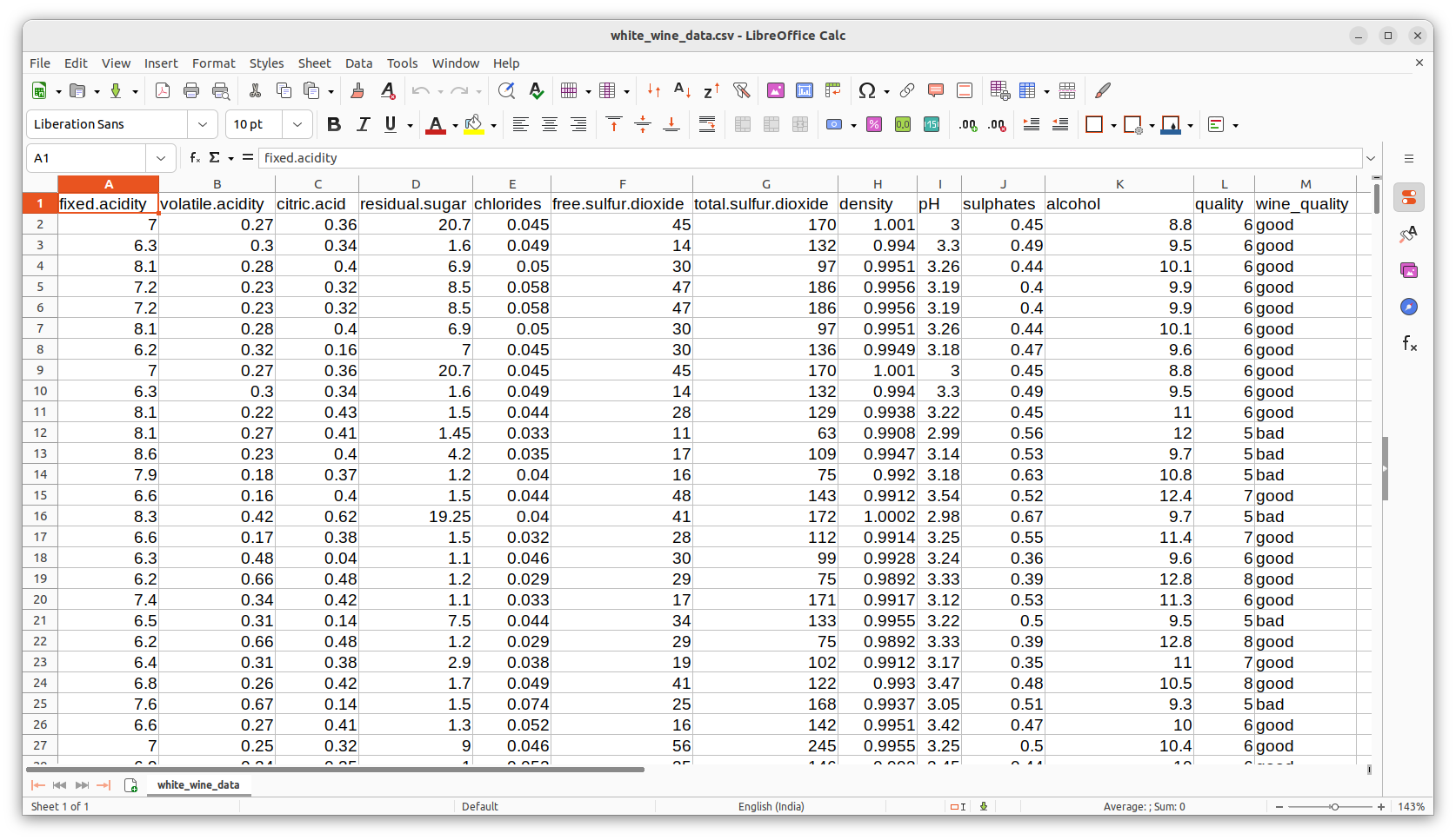
In R, the liogistic regression can be performed by the stats libray function called glm(). This function is used to fit generalized linear models, including logistic regression. The function call with essential parameters is:

glm(formula, family, data, weights, ....)


where,



 formula ----------> A symbolic description of the model to be fitted.

                        For example, "y ~ X1 + X2 + X3". Here, y is the vector on independent
			
			binary variable abd X1,X2 and X3 are dependent variables.


      Example formula :  

  For example, if Y is the independent binary variable and X1, X2, X3 are the three dependent 
  variables which are continuous, the formula is written as,
	           
		   Y ~ X1 + X2 + x3

  Suppose, if X1 is categorical and X2, X3 are continuous, then formula is written as,

	           Y ~ factor(X1) + X2 + X3

     where the factor() informs R that the variable X1 is categorical.



 family  ----------> a description of the error distribution and link function to
                        be used in the model. For binomial logistic regression, "family=binomial".

 data -----------> data frame with X and Y variables, whose names are used

                        in the formula above.

 weights  ----------> an optional vector of ‘prior weights’ to be used in the
          fitting process.  Should be ‘NULL’ or a numeric vector.

The R script presented below reads the data file white_wine_data.csv and performs logistic regression.

The above data set is available at the UC Machine learning repository and can be downloaded from "https://archive.ics.uci.edu/dataset/186/wine+quality"

For a large number of winw samples, values of 10 observaed dependent variables namely "fixed_acidity", "volatile_acidity", "citric_acid", "residual_sugar", "chlorides", "free_sulfur_dioxide", "total_sulfur_dioxide", "density", "pH" and "sulphates" are presented with an independent binary variable "wine_quality" with 2 possible values "good" or "bad".

The screen capture of a porion of data file is shown below:




In the R-script below, we read the file into a data frame and convert the "good" and "bad" outcomes of the wine_quality column into binary nubers 0 and 1 respectively. We then call the glm() function to perform the logistic regression. The output column is added to the original data set and written into a file "

## Model logistic regression analysis

dat = read.csv(file="white_wine_data.csv", header=TRUE)


## Take a subset of data
subdat=dat    ## all the 4898 rows included

## use this if need to use only subsets of data
#subdat = dat[1:2000,] ## only 2000 rows included
#subdat = dat[1:1000,] ## only 1000 rows included
#lsubdat = dat[1:200,] ## only 200 rows included


## convert the binary values of wine_quality to good=1, bad=0
wine_quality_num =  rep(0, nrow(subdat))


for( i in 1:length(subdat$wine_quality)){
  if(subdat$wine_quality[i] == "good"){ 
    wine_quality_num[i] = 1
  }

  if(subdat$wine_quality[i] == "bad"){
    wine_quality_num[i] = 0
  }

}

subdat = data.frame(subdat, wine_quality_num)


 ## Performing Logistic regression
glm.fit  =  glm(wine_quality_num ~ fixed.acidity + citric.acid + residual.sugar + free.sulfur.dioxide + total.sulfur.dioxide 
	     + density + pH + sulphates + alcohol,  data = subdat, family = binomial)


print(summary(glm.fit))


## other results
#confint(glm.fit) # 95% CI for the coefficients
#exp(coef(glm.fit)) # exponentiated coefficients
#exp(confint(glm.fit)) # 95% CI for exponentiated coefficients
#predict(glm.fit, type="response") # predicted values
#residuals(glm.fit, type="deviance") # residuals


##---------------------------------------------------------------------------

### Computing the fitted values and the probability og Y=1 given a set of X values

## exponent = b0 + b1*X1 + b2*X2 + ....+ bp*Xp
 Yex = rep(0, nrow(subdat))

## Probability that Y=1 for a given data points X.
 P = rep(0, nrow(subdat))


 Yex =  glm.fit$coefficients[1] + glm.fit$coefficients[2]*subdat$fixed.acidity 
              + glm.fit$coefficients[3]*subdat$citric.acid 
              + glm.fit$coefficients[4]*subdat$residual.sugar
	      + glm.fit$coefficients[5]*subdat$free.sulfur.dioxide 
	      + glm.fit$coefficients[6]*subdat$total.sulfur.dioxide 
	      + glm.fit$coefficients[7]*subdat$density 
	      + glm.fit$coefficients[8]*subdat$pH 
	      + glm.fit$coefficients[9]*subdat$sulphates 
	      + glm.fit$coefficients[10]*subdat$alcohol

## same result as above, easily using the function "predict()"
#Yex = predict(glm.fit)


## Compute the probability (Y=1|x values)
P = exp(Yex)/(1 + exp(Yex))

## same probabilities, using predict function with type=response
#P = predict(glm.fit, type="response")


## Write the results and original data into a data frame:
df = data.frame(subdat, P)

## write the data frame into a file.
write.csv(df, file="fitted_data.csv", row.names=FALSE)

##---------------------------------------------------------------------

Running the above script in R prints the following output lines and graph on the screen:

Call:
glm(formula = wine_quality_num ~ fixed.acidity + citric.acid + 
    residual.sugar + free.sulfur.dioxide + total.sulfur.dioxide + 
    density + pH + sulphates + alcohol, family = binomial, data = subdat)

Deviance Residuals: 
    Min       1Q   Median       3Q      Max  
-2.9443  -1.0271   0.4601   0.8652   2.4577  

Coefficients:
                       Estimate Std. Error z value Pr(>|z|)    
(Intercept)           3.549e+02  6.562e+01   5.409 6.34e-08 ***
fixed.acidity         1.615e-01  6.793e-02   2.377   0.0174 *  
citric.acid           8.022e-01  2.890e-01   2.776   0.0055 ** 
residual.sugar        1.955e-01  2.507e-02   7.798 6.30e-15 ***
free.sulfur.dioxide   1.703e-02  2.659e-03   6.405 1.50e-10 ***
total.sulfur.dioxide -5.199e-03  1.136e-03  -4.578 4.69e-06 ***
density              -3.708e+02  6.649e+01  -5.576 2.46e-08 ***
pH                    1.751e+00  3.396e-01   5.156 2.52e-07 ***
sulphates             2.061e+00  3.460e-01   5.958 2.56e-09 ***
alcohol               5.183e-01  8.677e-02   5.973 2.32e-09 ***
---
Signif. codes:  0 ‘***’ 0.001 ‘**’ 0.01 ‘*’ 0.05 ‘.’ 0.1 ‘ ’ 1

(Dispersion parameter for binomial family taken to be 1)

    Null deviance: 6245.4  on 4897  degrees of freedom
Residual deviance: 5214.3  on 4888  degrees of freedom
AIC: 5234.3

Number of Fisher Scoring iterations: 5

In the results of the logistic regression test shown above, the estimate of each coefficient is printed. For example, the value of itercept is 354.9 and the value of coefficient for fixed.acidity is 0.1615.

The column "z value" represents the Z-variable which is the ratio of estimated coefficient to its standard error.

The columnd titled $Pr(>|z|)$ gives the two sided probability of having a deviation greater than the observed Z-value. This probability should be compared to a choses significance value $\alpha$ to reject or accept the null hypothesis that the given coefficient is zero.

For example, if $\alpha=0.05$, then all the coefficients show a p-value less than this and hence retained. On the ohter hand, if we set $\alpha = 0.01$, then the null hypothesis for coefficient of "fixed.acidity" column is accepted since its p-value of 0.0174 which is greater than 0.01. This means that "fixed.acidity" does not play a significanr role in the model and hence can be removed from the model. All other coefficients are statistically significant and hence retained in the model.

Interpreting the results of Binary Logistic Regression

For a data with one or more predictor variables X and a binary response variable Y, the logistic regression analysis gives the probability of observing a state Y=1, given set of predictor variables.

Using this result, we can come up with two types of interpretations on the model.

1. Compute the change in odds of $Y=1$ for a unit change in X. Use this method to compute adjusted odds, ie, odds of Y=1 for a varible adjusted for other variables of the model.

2. Using the probability $P(y=1|\overline{x})$ for individual data points, use the model as a classifier that can classify every data point into one of the binary category (y=1/0) depending on the value of X.

Let us look at them in detail.

1. Interpreting the odds of an event

As an example, we consider a logistic regression model with two predictor variables $X_1$ and $X_2$ and an indepedent binary variable Y.

To begin with, we perform a logistic regression with only one predictor variable $x_1$ and get the result for the Odds(Y=1),

$odds(Y=1|X_1)~=\dfrac{P(Y=1|X_1)}{1-P(Y=1|X_1)}~=~{\Large e^{-3.20~+~0.522~X_1}}~~~~~~~~(1)$

Now, let us compute the Odds(Y=1) for a unit increase in the variable $X_1$ as,

$odds(Y=1|X_1 + 1)~=\dfrac{P(Y=1|X_1 + 1)}{1-P(Y=1|X_1+1)}~=~{\Large e^{-3.20~+~0.522~(X_1 + 1)}}~~~~~~~~(2)$

The odds ratio between two conditions is the ratio of odds of one condition with the odds of other condition.

Therefore, the odds ratio of $(Y=1|X_1)$ to $(Y=1|X_1+1)$ is obtained by dividing eqn(2) by eqn(1):

$odds~ratio~=~\dfrac{odds(Y=1|X_1 + 1)}{odds(Y=1|X_1)}~=~{\Large e^{0.522}}~=~1.68~~~~~~~~~~(3)$

For $X_1=3$ so that $X_1+1=4$, the the equation(3) states that "the odds of observing Y=1 for a predictor value of $X_1=4$ is 1.68 times higher than the odds of Y=1 for a predictor value of $X_1=3$". That is, the odds of Y=1 increases by $68\%$ per unit increase in $X_1$.


In the next step, we include the second variable $X_2$ in the analysis along with the first variable to perform the logistic regression. Suppose we get the result,

$odds(Y=1|X_1, X_2)~=\dfrac{P(Y=1|X_1,X_2)}{1-P(Y=1|X_1,X_2)}~=~{\Large e^{-3.61~+~0.435~X_1~+~0.712~X_2}}~~~~~~~~(4)$

In this case, the odds ratio $e^{0.435}~=1.55$ is interpreted as "the odds of Y=1 increases by 1.55 times per unit increase of $X_1$ adjusted for $X_2$".

Smilarly we can compute the odds ratio for a parameter adjusted for other parameters.

2. Using Logistic regression for classification

In the logisticregression analysis of a data set with n data points labelled as $i=1,2,3,...,n$ and p coefficients, the probability $p(Y_i=1|X_{i1},X_{i2},...,X_{ip})$ for the $i^{th}$ data point is obtained as,

$P(y_i=1|\overline{x_i})~=~\dfrac{\Large{e}^{b_0 + b_1 x_{i1} + b_2 x_{i2} + .....+ b_p x_{ip}} }{1~+~\Large{e}^{b_0 + b_1 x_{i1} + b_2 x_{i2} + .....+ b_p x_{ip}}}$






Thus, every data point gives a probability of Y=1 for a given set of values of X variables.

Suppose we set a threshold value of 0.5 for the probability.

If the model predicted P(Y=1) for a data point is above this threshold, we set Y=1 for the data point. Else we set Y=0.

Thus, we predict Y=0 or 1 for every data point accoeding to our fitted model. We say that our model is classifying the data point into one of the two binary categories of Y

For a set of X values, we can predict the binary status of Y (whether 0 or 1) according to our fitted logistic regression model using the equation above. By comparing these predicted Y values with the corresponding Y values from the observed data, we can quantify the predictive power of the model.

We call this "logistic regression as a classification method". We will see this in the "classification" section of the tutorial.

Multinomial Logistic Regression

In multinomial logistic regression, there are more than two classes for the dependent variable. it is no longer just binary. For example, based on various dependent variables like gender, age, income, family background, education etc, we want to predict whether a person in the starting of his career will buy a scooter, motor bike or a car. Here the scooter, bike and car are the three independent outcomes of the model.

In multinomial logistic regression, dependent variables are nominal(ie., the classes cannot be placed in any order) or ordinal(the classes can be placed in some order). Accordingly, the methods of regression vary. We will see both the cases here.

In multinomial logistic regression methods, the problem is transformed in such a way we perform many binary logistic regressions to combine the results. This is the general technique.

(A) Multinomial logistic regression with nominal dependent variables

There are two methods of performing multinomial logistic regression with nominal dependent variable:

(A1) K models for K classes

In this method, we will develope one binary logistic regression model for each class (possible outcome). We will consider the classes one by one. While considering a class, if the outcome belongs to that class, we make Y=1, and if it belongs to any of ramining classes, we make Y=0 to perform a binomial logistic regression. We repeat this for all the classes to get the probability of getting each class for every data point. For a given data point, we will assign the class for which the probability is maximum.

For example, let there be three classes(possible outcomes) namely A, B and C for the dependent variable Y.

Let $\overline{X}~=~\{ X_1, X_2, ...., X_p\}$ be the independent variables.

We develope a binary logistic regression model called "model A" with Y=1 if the outcome of a data point is A and Y=0 if the outcome is not A (it can be B or C)

This model gives us the probability $p(A)~=~P(Y=1~~in~model~A | \overline{X})$

Then we develope a binary logistic regression model called "model B" with Y=1 if the outcome of a data point is B and Y=0 if the outcome is not B (it can be A or C)

This model gives us the probability $p(B)~=~P(Y=1~~in~model~B| \overline{X})$

Lastly, we develope a binary logistic regression model called "model C" with Y=1 if the outcome of a data point is C and Y=0 if the outcome is not C (it can be A or B)

This model gives us the probability $p(C)~=~P(Y=1~~in~model~C| \overline{X})$

Thus, for each data point, we get three probabilities p(A), p(B) and p(C). We assign the class with highest probability to this data point.

For example, for a data point i, if $p(B) \gt p(C) \gt p(A)$, then the possible outcome is 'B'

Same method can be extended for any number of possible outcomes A,B,C,D,.... for the independent variable Y.

(A2) Simultaneous models in pairs

In this method, a binary logistic regression model is develped for the ratio of probabilities of two outcomes. For k possibilities, this give rise to k-1 binary logistic regression models of ratios. From this, probabilities for each possibility can be obtained.

For example, consider a model with three outcomes A, B and C described in the previous section.

For A and C, we develope a binary logistic regression model

$~~~log \left(\dfrac{p(A)}{p(C)}\right)~=~ a_1 + b_1^A x_1 + b_2^A x_2 + ....+ b_p^A x_p $

From this, we get

$~~p(A) ~=~ p(C)~{\Large e^{a_1 + b_1^A x_1 + b_2^A x_2 + ....+ b_p^A x_p}}~~~~~~~~~~~~~$(1)

Similarly, for B and C we develope a model,

$~~~log \left(\dfrac{p(B)}{p(C)}\right)~=~ a_2 + b_1^B x_1 + b_2^B x_2 + ....+ b_p^B x_p $

From this, we get

$~~p(B) ~=~ p(C)~{\Large e^{a_2 + b_1^B x_1 + b_2^B x_2 + ....+ b_p^B x_p}}~~~~~~~~~~~~~$(2)

Since A,B,C are mutuallu exclusive and mutually exhaustive outcomes, we have

$p(A)+p(B)+p(C)~=~1~~~~~~~~~$(3)

Substituting for p(A) and p(B) from (1) and (2) in (3), we get anexpression for computing p(C) in terms of coefficients of the two logistic regression models we built.

Once we get p(C), we can successively get p(A) and p(B) from equations (1) and (2). Thus we have p(A), p(B) and p(C) for every data point $(y_i, \overline{X}_i)$. We can assign the class A,B or C which has maximum probability.

Performing Multinomial Logistic Regression with nominal dependent variables in R

In R, The multinomial logistic regression with nominal dependent variable can be performed with "multinorm()" function of "nnet" package. "nnet"package in R performs logistic regression using neural network method. The essential parameters of the funtion multinom() are

  multinom(formula, data, weights, subset) 


 where,



 formula ----------> A symbolic description of the model to be fitted.

                        For example, "y ~ X1 + X2 + X3". Here, y is the vector on independent
			
			binary variable abd X1,X2 and X3 are dependent variables.


 data  is the data frame with above named columns

 weights  : optional case weights in fitting.

 subset  : expression saying which subset of the rows of the data should
          be used in the fit. All observations are included by default.

The R script presented below reads the data file multinomial_logistic_regression_nominal_data_simulated.csv and performs logistic regression.

This table contains 4 independent variables X1, X2, X3 and X4 and an independent variable Y which is multinomial with three nominal categories "A", "B" and "C". In this analysis, we keep the category "C" as the reference.

## Performing Multinomial Logistic Regression with ordinal idependent variables using R

## For this, we use "multinorm()" function of "nnet" package in R.
## Note:  "nnet"package in R performs logistic regression using neural network method.

library(nnet)

simdat = read.csv(file="multinomial_logistic_regression_nominal_data_simulated.csv", header=TRUE)

## convert Y categories to factor
simdat$Y = as.factor(simdat$Y)

# define reference by ensuring it is the first level of the factor
# The levels of a factor are re-ordered so that the level specified
#    by ‘ref’ is first and the others are moved down

simdat$Y2 = relevel(simdat$Y, ref = "C")

# check that C is now our reference
print(levels(simdat$Y2))


## First, calculate the multinomial logistic regression model
## for this, we use "multinom()" function of nnet package

multinomial_model = multinom(formula =  Y2 ~ X1 + X2 + X3 + X4,  data = simdat )



print(summary(multinomial_model))

	           
##

# calculate z-statistics of coefficients
z_stats = summary(multinomial_model)$coefficients/summary(multinomial_model)$standard.errors

# convert to p-values
p_values = (1 - pnorm(abs(z_stats)))*2

cat("", sep="\n")
cat("", sep="\n")

print("p-values for coefficient estimation:")

# display p-values in transposed data frame
print( data.frame(t(p_values)) )

cat("", sep="\n")
cat("", sep="\n")

print("Odds Ratios : ")
# display odds ratios in transposed data frame
odds_ratios = exp(summary(multinomial_model)$coefficients)
print( data.frame(t(odds_ratios)) )

cat("", sep="\n") # prints a blank line as seperator
cat("", sep="\n")


## get the coefficients of the model
# print(coef(multinomial_model))

cat("", sep="\n") # prints a blank line as seperator
cat("", sep="\n")

print("Predicted Probabilities for first 10 data points:")


## get the predicted probabilities of the model
predicted_prob = fitted(multinomial_model)
print(predicted_prob[1:10,])

Running the above script in R prints the following output lines and graph on the screen:

[1] "C" "A" "B"
# weights:  18 (10 variable)
initial  value 5493.061443 
iter  10 value 4488.581344
final  value 4292.030528 
converged
Call:
multinom(formula = Y2 ~ X1 + X2 + X3 + X4, data = simdat)

Coefficients:
  (Intercept)         X1        X2         X3         X4
A    2.561344 -0.6926831 -1.869736 -0.2481890  0.2668859
B   -1.954537 -0.1679250  1.129060  0.2675787 -0.2567193

Std. Errors:
  (Intercept)         X1         X2         X3         X4
A   0.3664625 0.08613650 0.08314800 0.07140571 0.10860615
B   0.3048346 0.06923229 0.05514513 0.05817441 0.08810575

Residual Deviance: 8584.061 
AIC: 8604.061 


[1] "p-values for coefficient estimation:"
                       A            B
(Intercept) 2.761125e-12 1.438174e-10
X1          8.881784e-16 1.528605e-02
X2          0.000000e+00 0.000000e+00
X3          5.094108e-04 4.233130e-06
X4          1.399571e-02 3.571010e-03


[1] "Odds Ratios : "
                     A         B
(Intercept) 12.9532153 0.1416301
X1           0.5002321 0.8454172
X2           0.1541644 3.0927473
X3           0.7802125 1.3067965
X4           1.3058914 0.7735853




[1] "Predicted Probabilities for first 10 data points:"
           C          A          B
1  0.1706570 0.78233869 0.04700434
2  0.4554722 0.16552473 0.37900309
3  0.3131811 0.52972904 0.15708985
4  0.1714166 0.00978960 0.81879377
5  0.4562092 0.19500801 0.34878278
6  0.3547093 0.42300470 0.22228599
7  0.2619757 0.02723238 0.71079189
8  0.3756347 0.28635280 0.33801253
9  0.4577073 0.27739574 0.26489697
10 0.2572670 0.00964465 0.73308833
> 

We understand and interpret the above results.

In this analysis, we have have modelled the nominal outcomes A and B with reference to C.

The independent variables are X1, X2, X3 and X4.

By looking at the block titled "Coefficients", we get the Coefficients for constant term, X1, X2, X3 and X4 for the two cases. We write the models in terms of log odds as,

$log \left ( \dfrac{P(A)}{P(C)} \right ) ~=~ 2.5613 - 0.69268 ~X1 - 1.8697 ~X2 - 0.24819 ~X3 + 0.2669 ~X4$

$log \left ( \dfrac{P(B)}{P(C)} \right ) ~=~ -1.9545 - 0.16792 ~X1 + 1.1291~X2 + 0.2676~ X3 - 0.2567 ~X4 $

We observe that the p-values of all the coefficients are significantly smaller. So, all the independent variables are important in the model.

The interpretations of coefficients are as follows (we have given few examples):

(1) A one-unit increase in the variable X1 is associated with the decrease in the log odds of being in C Vs. A by an amount of 2.56

(2) A one-unit increase in the variable X1 is associated with the decrease in the log odds of being in B Vs. C by an amount of 0.16

(B) Multinomial logistic regression with ordered category of dependent variables (Proportional odds logistic regression)

In some data, the categorical outcomes are ordinal, ie., they can be placed in an order. One simple example is the income groups classified into four categories of incresing order like "low income", "medium income", "high income" and "rich". We perform ordinal logistic regression for this type of data. This is also called as proportional odds logistic regression, which will be described in detail in this section.

[ Reference : Some of the steps described in this section were adopted from Chapter 7 of the lucidly written book titled "Handbook of Regression Modeling in People's Analytics with examples in R and Python" by Keith McNulty, published by Chapman & Hall/CRC, available in web version at "https://peopleanalytics-regression-book.org/index.html". ]


In real life data, the ordered categories of data are obtained by applying thresholds at various points on a continuous scale. In the above example, though individuals earn a wide range of income from very low to very high, the categories like "low income", "medium income" and "high income" are created by applying thresholds on the income scale.

In order to understand the proportional odds regression, we start with a dependent variable $y'$ that is continuous and dependent on a single continuous variable $x$. We arrive at a logistic model by categorizing the continuous variable $y$ with some thresholds.

Suppose we categorize the continuous variable $y$ using threshold values denoted by $t_1$, $t_2$, $t_3$ etc.

We define a discrete variable $y$ in terms of thresholds on $y'$ as,

$~~~~y~=~1$ when $~y' \leq t_1$
$~~~~y~=~2$ when $~t_1 \lt y' \leq t_2$
$~~~~y~=~2$ when $~t_2 \lt y' \leq t_2$
...........etc.......

For every threshold on $y'$, we assume a logistic regression model.

For example, when $y' \leq t_1$, we can set up a logistic regression model for $P(y=1 | x)$ between y and x. Same thing can be done for other values of y.

In a linear regression, we modela linear continuous variable as,

$~~~y'~=~\beta_0 + \beta_1 x + \epsilon '~~~~~~~~~~(1)$

where $\beta_0, \beta_1$ are the coefficients and $\epsilon '$ is the error term assumed to be a Gaussian variable.

In the logistic regression, we assume that

$~~y'~=~\beta_0 + \beta_1 x + \sigma \epsilon$

where where $\beta_0, \beta_1$ are the coefficients, $\sigma$ is proportional to the varince of $y'$ and $\epsilon$ is the error term.

The error term $\epsilon$ is assumed to follow the shape of a logistic function given by,

$~~~P(\epsilon \leq z)~=~\dfrac{1}{1 + \large{e}^{-z}}~~~~~~~~~~~~(2)$

$~~~~~~~~~~~~~~~~~~~~$
$~~~~~~~~~~~~~~~~~~~~$
$~~~~~~~~~~~~~~~~~~~~~~~~~~~~~~~{\large Note} $

The above mentioned logistic function used as error term is the cumulative distribution function of a symmetric probability distribution called Standard Logic Distribution given by,

$~~~~~~~f(z)~=~\dfrac{\large e^z}{({\large e^z} + 1)^2} ~~~~$ with $-\infty \lt z \lt \infty$

The Cumulative Density Function (CFD) of the above standard logistic distribution upto any value $z$ is obtained by integrating it from -$\infty$ to $z$.


$~~~~~~F(z)~=~\displaystyle \int_{-\infty}^{z} \dfrac{\large e^z}{({\large e^z} + 1)^2} dx ~=~\dfrac{1}{1 + \large{e}^{-z}}$ $~~~~~~~~~~~~~~~~~~~~$
$~~~~~~~~~~~~~~~~~~~~$
The probability that our ordinal variable $y$ is at the state $y=1$ is given by,

$P(y=1)~=~P(y' \leq t_1) $

$~~~~~~~~~~~~~~~~~=~P(\beta_0 + \beta_1 x + \sigma \epsilon \leq t_1) $

$~~~~~~~~~~~~~~~~~=~P(\epsilon \leq \dfrac{t_1 - \beta_0 - \beta_1 x }{\sigma}) $

$~~~~~~~~~~~~~~~~~=~P(\epsilon \leq \tau_1 - \beta x)~~~~~~~~~~~$ with $~~~~\tau_1 = \dfrac{t_1 - \beta_0}{\sigma}~~~$ and $~~\beta = \dfrac{\beta_1}{\sigma}$

Using the equation (2) above, we write

$~~~~~~~P(y=1)~~~~=~\dfrac{1}{1 + \large{e}^{- (\tau_1 - \beta x) }}~~~~~~~~~~~~~~~(3)$

We can also write,

$ P(y \gt 1)~=~1 - P(y=1)~=~1~-~\dfrac{1}{1 + \large{e}^{- (\tau_1 - \beta x) }} ~=~\dfrac{\large{e}^{- (\tau_1 - \beta x) }}{1 + \large{e}^{- (\tau_1 - \beta x) }}~~~~~~(4) $

Using Equations (3) and (4), we compute the ratio

$~~~~~~~~~~~~~~~~~~\dfrac{P(y=1)}{P(y > 1)} ~=~{\large{e}^{\tau_1 - \beta x}}~~~~~~~~~~~(5) $

Taking logarithm on both sides,

$~~~~~~~~~~~~~~~~~log{\displaystyle \left(\dfrac{P(y=1)}{P(y \gt 1)}\right)}~=~{\large \tau}_1 - \beta x ~~~~~~~~~~~~~(6)$

is the log odds that the ordinal outcome is in the category cprresponding to $y=1$.

Following the same line of arguments, we can derive the log odds of our ordinal outcome to be in the next category $y=2$ as,

$~~~~~~~~~~~~~~~~~log{\displaystyle \left(\dfrac{P(y \leq 2)}{P(y \gt 2)}\right)}~=~{\large \tau}_2 - \beta x ~~~~~~~~~~~~~(6)$

where $~~~~\tau_2 = \dfrac{t_2 - \beta_0}{\sigma}~~~$ and $~~\beta = \dfrac{\beta_1}{\sigma}$

This method can be generalized to an arbitrary number of ordinal categories indexd by the letter k to write,

$~~~~~~~~~~~~~~~~~log{\displaystyle \left(\dfrac{P(y \leq k)}{P(y \gt k)}\right)}~=~{\large \tau}_k - \beta x$

{\large \tau}_k where $~~~~\tau_k = \dfrac{t_k - \beta_0}{\sigma}~~~$ and $~~\beta = \dfrac{\beta_1}{\sigma}$


$~~~~~~~~~~~~~(7)$






Alternatively, we can also write

$~~~~~~~~~~~~~~~~~log{\displaystyle \left(\dfrac{P(y \gt k)}{P(y \leq k)}\right)}~=~-({\large \tau}_k - \beta x)~=~\beta x - {\large \tau}_k$

$~~~~~~~~~~~~~(8)$


Let us look at the Equation(8) above more carefully. According to this equaition, the relation between log odds in favour of $y \gt k$ and the independent variable x is a straight line with slope $\beta$ and intercept $\tau_k$. This slope $\beta$ is same for all the categories k.

Therefore we can state that for a unit change in $x$, the log odds in favour of $y \gt k$ is $\beta$. This is true for every category k.

We realize that each unit increase in x increses the log odds of y being in a higher category by a constant ratio

This is why we call this "Proportional odds Regression"

General forms of Proportional odds regression model

We extend the above concept to a proportional odds logistic regression of a data with k discrete possible states of dependent variable y and p independent variable denoted by $x_1, x_2, x_3,....,x_p$.

There are three ways in which the proportional odds model can be parametrized:

$log{\displaystyle \left(\dfrac{P(y \leq k)}{P(y \gt k)}\right)}~=~\alpha_k - (\beta_1 x_1 + \beta_2 x_2 + \beta_3 x_3 + ....+\beta_p x_p)~~~~~~~~$ (Model-1)

$log{\displaystyle \left(\dfrac{P(y \leq k)}{P(y \gt k)}\right)}~=~\alpha_k + (\beta_1 x_1 + \beta_2 x_2 + \beta_3 x_3 + ....+\beta_p x_p)~~~~~~~~$ (Model-2)

$log{\displaystyle \left(\dfrac{P(y \gt k)}{P(y \leq k)}\right)}~=~\alpha_k + (\beta_1 x_1 + \beta_2 x_2 + \beta_3 x_3 + ....+\beta_p x_p)~~~~~~~~$ (Model-3)

In Model-1 and Model-3, for positive values of $\beta$, as the value of the explanatory variable increases, the likelihood of lower ranking decreases and hence the likelihood of higher ranking increases. Wheras, in Model-2, for the positive value of $\beta$, as the value of the explanatory variable increases, the likelihood of lower ranking increases and hence the likelihood of higher ranking decreases.

Performing proportional odds logistic regression in R

The proportional odds logistic regreesion for ordinal outcomes of dependent variable can be performed with the "clm()" function of the "ordinal" library in R.

The "clm()" function Fits cumulative link models (CLMs) such as the propotional odds model. The essential parameters of the funtion clm() function are

  clm(formula, data, weights,...) 


 where,



 formula ----------> A symbolic description of the model to be fitted.

                        For example, "y ~ X1 + X2 + X3". Here, y is the vector on independent
			
			binary variable abd X1,X2 and X3 are dependent variables.


 data  is the data frame with above named columns

 weights  : optional case weights in fitting.

The R script presented below reads the data file multinomial_logistic_regression_ordinal_data_simulated.csv and performs logistic regression.

This table contains 4 independent variables X1, X2, X3 and X4 and an independent variable Y which is ordinall with four states "A","B","C","D". (Here, A < B < C < D )

## Perform ordinal logistic regression on data set df using "ordinal"package of R.


 library(ordinal)

 dat = read.csv(file="multinomial_logistic_regression_ordinal_data_simulated.csv", header=TRUE)

 dat$Y = as.factor(dat$Y)


 model = clm(Y ~ X1 + X2 + X3 + X4, data = dat)

 print(summary(model))
 

Running the above script in R prints the following output lines and graph on the screen:

 
formula: Y ~ X1 + X2 + X3 + X4
data:    dat

 link  threshold nobs logLik   AIC     niter max.grad cond.H 
 logit flexible  5000 -3220.75 6455.50 7(1)  8.01e-13 4.0e+03

Coefficients:
   Estimate Std. Error z value Pr(>|z|)    
X1  0.74775    0.07549   9.906  < 2e-16 ***
X2  2.05167    0.06854  29.934  < 2e-16 ***
X3  0.39702    0.06198   6.406 1.49e-10 ***
X4 -0.36218    0.09506  -3.810 0.000139 ***
---
Signif. codes:  0 ‘***’ 0.001 ‘**’ 0.01 ‘*’ 0.05 ‘.’ 0.1 ‘ ’ 1

Threshold coefficients:
    Estimate Std. Error z value
A|B   1.4836     0.3172   4.678
B|C   2.0181     0.3176   6.354
C|D   2.5356     0.3186   7.958