CountBio
Mathematical tools for natural sciences
Biostatistics with R
Multiple plots on the same page
We can draw more than one plot on the same canvas using the
This function can be used to set or query graphical parameters. A call to
For example, the following call to par() will create an empty canvas on the screen into which we can draw 4 plots, in 2x2 format:
par(mfrow = c(2,2))
The parameter value mfrow = c(2,2) divides the canvas into 2x2 sections and plots the 4 graphs successively along the rows. Thus, firat 2 plots will be on first row, next two will be on second row. Similarly, the option mfcol = c(2,3) divies the canvas into 2 row and 3 columns. Six successive plots following the call will be filled along columns.
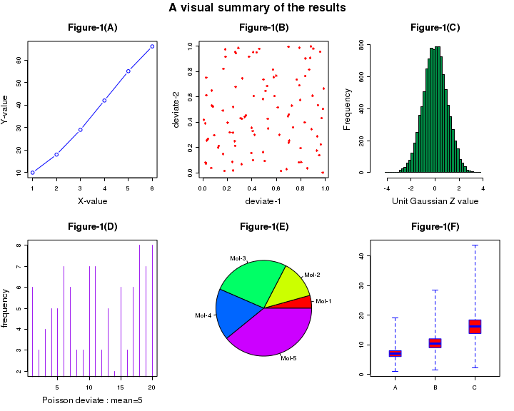
The code shown below demonstrates a multiple plot. The data points are generated using random deviate functions in R. The comments before each code line explains the function called for the plot.
# This script demonstrates multiple plots in a single figure.

##  Set up plotting in two rows and three columns.
##  Set the outer margin for bottom, left, and right as 0 and
##  outer margin for top is 2 lines of text.
##  Plotting goes along rows first.
##  To plot along columns, usde "mfcol" instead of mfrow.
par( mfrow = c( 2, 3 ), oma = c( 0, 0, 2, 0 ) )

## Call the first plot. This is drawn at the location row 1, column 1:
## simple (X,Y) plot
plot(c(1,2,3,4,5,6),c(10,18,29,42,55,66), type="b", col="blue", main="Figure-1(A)",
             xlab="X-value", ylab="Y-value")

## Call the second plot. This is drawn at the location row 1, column 2:
## We generate 2 sets of 100 uniform random numbers and create their scatter plot.
## "runif(100)" returns 100 uniform random numbers between 0 and 1.
plot(runif(100), runif(100), col="red", pch = 8, xlab="deviate-1",
          ylab="deviate-2", main="Figure-1(B)")

##Call the third plot. This is located in row 1, column 3:
## "rnorm(10000)"generate a histogram of 10000 gaussian deviates
hist(rnorm(10000), breaks=30, col="springgreen4", xlim = c(-5,5), xlab="Unit Gaussian Z value",
          ylab="Frequency", main="Figure-1(C)")

## Call the fourth plot. It is located in row 2, column 1:
## We generate 20 poinrs from a Poisson distribution and plot them.
plot( rpois(n=20, lambda=5), type = "h", col="purple", xlab="Poisson deviate : mean=5",
          ylab="frequency", main="Figure-1(D)")

##  plot.new() skips a position, if needed.


##  The fifth plot is located in row 2, column 2:
# Create a Pie chart with a heading and rainbow colors
result <- c(10, 30, 60, 40, 90)
pie(x = result, main="Figure-1(E)", col=rainbow(length(result)),
               label=c("Mol-1","Mol-2","Mol-3", "Mol-4", "Mol-5"))

## The sixth plot is located in row 2, column 3
# we create a list of vectors and call box plot with it.
# Three Box-Whiskers are plotted, for x, y and x vectors
x <- c(1,5,7,8,9,7,5,1,8,5,6,7,8,9,8,6,7,8,10,19,6,7,8,6,4,6)
y = x*1.5
z = x*2.3
alis <- list(x,y,z)
boxplot(alis, range=0.0, horizontal=FALSE, varwidth=TRUE, notch=FALSE,
        outline=TRUE, names=c("A","B","C"), boxwex=0.3,
        border=c("blue","blue","blue"), col=c("red","red","red"), main="Figure-1(F)")

# Title is given to the whole of the plot.
title("A visual summary of the results", outer=TRUE)
To skip a plot in par()
While plotting multiple plots using par(), sometimes we want to skip a plot in the matrix and leave a blank space in its location. This can be achived using the call to Multiple plots by splitting the screen
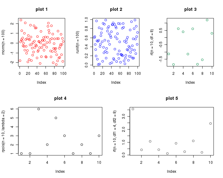
Another way of creating multiple plots on the same screen is by splitting the screen into regions and plotting. We use
We first split the screen into rows. Each row in turn is split into as many sections as required. In this way, different rows can have different number of figures.
As an example, suppose we want to place three figures along first row and two figures below them on the second row. We proceed as follows:
which splits the screen into 2 rows and 1 column. We get screens 1(top) and 2(bottom). We can further split the top and bottom screen again. For example, command below splits screen 1 (top screen) into one row and three columns. We get screens 3,4,5:
We now split bottom screen (screen 2) into 2 columns to get screen 6 and 7:
If we now create 5 plots one by one, plots are placed from screen 3 to 7. Thus we get 3 plots on top row, and 2 on bottom row, as we wished. See the code below, which is self explanatory because of comments.
##  Split the screen into two rows and one column, defining screens 1 and 2.
split.screen( figs = c( 2, 1 ) )

##  Split screen 1 into one row and three columns, defining screens 3, 4, and 5.
split.screen( figs = c( 1, 3 ), screen = 1 )

##  Split screen 2 into one row and two columns, defining screens 6 and 7.
split.screen( figs = c( 1, 2 ), screen = 2 )

##  The first plot is located in screen 3 (first row):
screen( 3 )
plot( rnorm( n = 100 ), col = "red", main = "plot 1" )

##  The second plot is located in screen 4 (first row):
screen( 4 )
plot( runif( n = 100 ), col = "blue", main = "plot 2" )

##  The third plot is located in screen 5 (first row):
screen( 5 )
plot( rt( n = 10, df = 8 ), col = "springgreen4", main = "plot 3" )

##  The fourth plot is located in screen 6 (second row):
screen( 6 )
plot( rpois( n = 10, lambda = 2 ), col = "black", main = "plot 4" )

##  The fifth plot is located in screen 7 (second row):
screen( 7 )
plot( rf( n = 10, df1 = 4, df2 = 8 ), col = "gray30", main = "plot 5" )

##  Close all screens.

close.screen( all = TRUE )