CountBio
Mathematical tools for natural sciences
Basic Statistics with R
Geometric distribution
The binomial distribution computes the probability of getting \( x \) successes in a sequence of \( n\) Bernoulli trials. We ask the following question: if \(p\) is the probability of success in each trial, how many trials we have to perform until we observe the first success?
Let the first success occur in the \( x^{th} \) trial. This \( x \) follows a geometric distribution
Suppose we perform a sequence of Bernoulli trials and note down the \( x^{th} \) trial when first success occurs.
For example, let ’S’ denote success and ’F’ denote failure in a Bernoulli experiment. We perform the experiment many times to get a sequence FFFFSFSS.... Here the first success occurs on fifth trial and hence \( x = 5 \). If we repeat these trials again and get a sequence FFSFSSFFSF...., we have \( x=3 \).
If we repeat this experiment many many times, what will be distribution of \(x\)?.
We will derive an expression for the probability distribution function of geometric distribution as follows.
If \(p\) is the probability of success and \(1-p\) is the probability of failure in a single Bernoulli trial,
\(\small{P(x)~=~P(first~success~on~trial~x) } \) \(\small{~~~~~~~~=~P(first~x-1~trials~result~in~failure~and~x^{th}~trial~a~success) } \) \(\small{~~~~~~~~=~P(first~x-1~trials~result~in~failure) \times P(x^{th}~trial~a~success) } \) \(\small{~~~~~~~~=~(1-p)^{x-1} \times p } \)
Therefore, the probability density function of geometric distribution that gives the probability of observing the first success on \(x^{th}\) trial, with \(p\) being the probability of success for each trial is given by ,
Why the name "Geometric distribution"?
The Geometric series is given by, \( ~~~~~~~~~~~~~~~\small{ \sum\limits_{k=0}^n ar^k~=~a + ar + ar^2 + ar^3 + ar^4 + ....}\) where the series converges for \( \small{-1 \leq r \leq 1 }\).
Now consider the summation of the geometric distribution expression with \( k = x-1 \): \(~~~~~~~~\small{\sum\limits_{x=1}^n p(1-p)^{x-1} = \sum\limits_{k=0}^{n-1} p(1-p)^{k} }\) With p=a, 1-p = r and n-1 = m, the above expression resembles a geometric progression \( \small{\sum\limits_{k=0}^m ar^k } \). hence the name geometric distribution
The mean and variance of the Geometric distribution
The expressions for the mean and the variance of the geometric distribution are given below (derivation not shown):
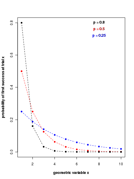
The plot of Geometric probability distribution
The figure below shows the probability density plots of geometric distribution for various values of probability of success \( p \).
R scripts
The R statistics library provides the following four basic functions for the geometric distribution.
x = trial number at which the first success is observed (ie., first success after x-1 successive failures)p = probability of success in a trialdgeom(x,p) -----> Returns the probability density for success in trial number x.pgeom(x,p) -----> Returns the cumulative geometric probability for x=1 upto value of x.qgeom(pvalue, p) -----> Inverse of the pgeom() function. Returns the x value upto which the cumulative probability is pvalue (quantiles).rgeom(n, p) -----> Returns n random deviates from a hypergeometric distribution with the probability of success p.
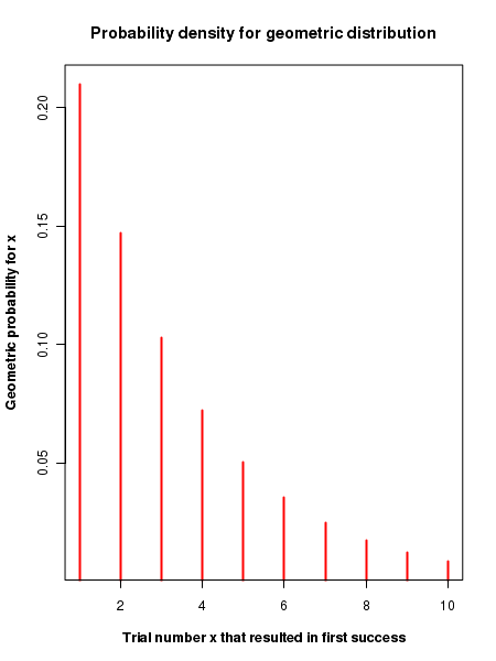
### Generating the probability density function of geometric distribution

x = seq(1,10)
p = 0.3
y =  dgeom(x,p)
plot(x,y,type="h", col="red", lwd=2, xlab="Trial number x that resulted in first success",
          ylab = "Geometric probability for x", font.lab=2,
	  main="Probability density for geometric distribution")

## Computing cumulative probability upto x=4
p = 0.2
x = 4
prob = pgeom(x,p)
print(paste("Cumulative probability of geometric distribution upto x=4 = ",
                round(prob, digits=3)))

## Computing value of x at which cumuative probability crosses q
p = 0.2
pcumul = 0.738
xval = qgeom(pcumul, p)
print(paste("trial number x value at which cumulative probability crosses pcumul = ", xval))

## Generating 6 random deviates from geometric distribution
p = 0.4
x = rgeom(6, p)
print("some random deviates from geometric distribution with p=0.4 : ")
print(round(x, digits=3))
Running the above script in R prints the following output lines and graph on the screen:
[1] "Cumulative probability of geometric distribution upto x=4 =  0.672"
[1] "trial number x value at which cumulative probability crosses value 0.738 value =  6"
[1] "some random deviates from geometric distribution with p=0.4 : "
[1] 5 2 2 0 1 3