CountBio
Mathematical tools for natural sciences
Basic Statistics with R
Two sample t tests
These tests are used to compare the means of two populations which are normally distributed with unknown variances. When the varianes are not known and the sample sizes are large (> 30), we can use a two sample Z test for comparing the means, as explained in the previous section. However, when the sample sizes are small and the variances unknown, we use a t statistic to test the equality of two means.
Let X and Y be two data sets of n and m random samples respectively from normal distributions \(\small{N(\mu_X, \sigma_X)}\) and \(\small{N(\mu_Y, \sigma_Y)}\). Suppose the values of the variances \(\small{\sigma_X^2 }\) and \(\small{\sigma_Y^2 }\) are unknown. Three possibilities arise: \(~~~~~~~~~~\) (i) The two samples are idependent, population variances are unknown but assumed to be equal. \(~~~~~~~~~~\) (ii) The two samples are independent, population variances are unknown and unequal. \(~~~~~~~~~~\) (iii) The two samples are dependent. These three cases give rise to a family of t-tests which are described below:
1. Two sample t test for independent samples of unknown and equal population variances
We have learnt that, when the variances are unknown and equal, the difference between the means \(\small{\overline{X} }\) and \(\small{\overline{Y} }\) of the two independent samples of sizes n and m respectively is known to follow a t disribution of (n+m-2) degrees of freedom with a combined standard deviation \(\small{S_p}\). Computing the standard deviations \(\small{S_X}\) and \(\small{S_Y}\) of the two samples, we write the corresponding T statistic as, \(\small{ T = \dfrac{\overline{X} - \overline{Y} - (\mu_X - \mu_Y)}{\sqrt{\left[\dfrac{(n-1)S_X^2 + (m-1)S_Y^2}{n+m-2}\right] \left[\dfrac{1}{n} + \dfrac{1}{m}\right] } } ~~ = ~~ \dfrac{\overline{X} - \overline{Y} - (\mu_X - \mu_Y)}{S_p \sqrt{\left[\dfrac{1}{n} + \dfrac{1}{m}\right]}}}\) where the pooled standard deviation \(\small{S_p}\) is defined as, \(~~~\small{S_p = \sqrt{\dfrac{(n-1)S_X^2 + (m-1)S_Y^2}{n+m-2} } }\)
This T variable has a t distribution with (n+m-1) degrees of freedom denoted by t(n+m-2).Using the sample parameters, we construct an approxiamate \(\small{100(1-\alpha)}\) percent confidence interval for \(\small{\mu_X - \mu_Y }\) given by, \(\small{(\overline{X} - \overline{Y}) \pm t_{1-\frac{\alpha}{2}}(n+m-1) S_p \sqrt{\dfrac{1}{n} + \dfrac{1}{m} } }\)
This t variable is used as the test statistic for the two sample t test. The null hypothesis can be tested for three possibilities: \(~~~~~~~~\small{\mu_X - \mu_Y = 0,~~~~\mu_X - \mu_Y > 0~~and~~~\mu_X - \mu_Y < 0 }\). For all the three cases, the hypothesis will be tested at \(\small{\mu_X - \mu_Y = 0}\). Therefore, the t statistic for the test is written as, \(\small{ T = \dfrac{\overline{X} - \overline{Y}}{\sqrt{\left[\dfrac{(n-1)S_X^2 + (m-1)S_Y^2}{n+m-2}\right] \left[\dfrac{1}{n} + \dfrac{1}{m}\right] } } ~~ = ~~ \dfrac{\overline{X} - \overline{Y}}{S_p \sqrt{\left[\dfrac{1}{n} + \dfrac{1}{m}\right]}} }\)
Under the null hypothesis, this t statistics follows t distribution with (n+m-1) degrees of freedom. We can test a null hypothesis for a given significance level of \(\small{\alpha}\), using the following steps of hypothesis testing.
- We first compute the sample means \(\small{\overline{X}}\), \(\small{\overline{Y}}\) followed by the sample standard deviations \(s_X, s_Y \) from the data.
- Knowing the value of means and the standard deviations of two data sets, we compute the value of t statistic using the expression given before.
- The statistical significance (also called "p-value") of this data is then obtained by computing the probability \(\small{P(\gt t) }\) or \(\small{P(\lt -t })\) from the t distribution with (n+m-2) degrees of freedom. Under the null hypothesis, the p-value represents the probability of getting the observed statistic t.
- If the p-value is either smaller than a pre-decided value \(\small{\alpha}\) or the observed t statistic is outside a given range (\(\small{-t_0 \leq Z \leq t_0) }\), we reject the null hypothesis and accept the alternate hypothesis. Here, \(\small{t_0}\) is the value of statistic above which the area under the t distribution curve for (n+m-2) degrees of freedom is \(\small{\alpha}\).
- We can also reject the null hypothesis if the computed t statistic for the data is outside the \(\small{(1-\alpha)100\%}\) confidence interval on the population mean.
This test is used in the Example-1 at the end of this tutorial.
3. Two sample t test for independent samples of unknown and unequal population variances - The Welsch t test
We have learnt that When the two population variances are unknown and unequal, the quantity \(\small{t_w = \dfrac{\overline{X} - \overline{Y} - (\mu_X - \mu_Y)}{\sqrt{\dfrac{S_X^2}{n} + \dfrac{S_Y^2}{m}}} }\) approximately follows a student's t distribution with a modified degrees of freedom \(\small{r}\). An expression for this modifie degree of freedom is given by the Welch-Satterthwaite correction as,
\(~~~~~~~~~~~~~~~~\small{r = \dfrac{\left(\dfrac{s_X^2}{n} + \dfrac{s_Y^2}{m}\right)^2} {\dfrac{1}{n-1}\left(\dfrac{s_X^2}{n}\right)^2 + \dfrac{1}{m-1} \left(\dfrac{s_Y^2}{m}\right)^2 } }\)This t variable can be used as the test statistic for the two sample t test. The null hypothesis can be tested for three possibilities: \(~~~~~~~~\small{\mu_X - \mu_Y = 0,~~~~\mu_X - \mu_Y > 0~~and~~~\mu_X - \mu_Y < 0 }\). For all the three cases, the hypothesis will be tested at \(\small{\mu_X - \mu_Y = 0}\). Therefore, the t statistic for the test is written as, \(\small{t_w = \dfrac{\overline{X} - \overline{Y}}{\sqrt{\dfrac{S_X^2}{n} + \dfrac{S_Y^2}{m}}}~=~t(r), }\) a student's t distribution with r degrees of freedom. The \(\small{(1-\alpha)100\%}\) confidence intervl for the difference $\mu_X-\mu_Y$ is given by, \(~~~~~~~~~~~~~~~~~~~\small{(\overline{X} - \overline{Y}) \pm t_{1-\alpha/2}(r) \sqrt{\dfrac{S_X^2}{n} + \dfrac{S_Y^2}{m} } }\)
Under the null hypothesis, the test statistic follows t distribution with r degrees of freedom. We can test a null hypothesis for a given significance level of \(\small{\alpha}\), using the following steps of hypothesis testing.
- We first compute the sample means \(\small{\overline{X}}\), \(\small{\overline{Y}}\) followed by the sample standard deviations \(\small{s_X}\), \(\small{s_Y}\) from the data.
- Knowing the value of means and the standard deviations of two data sets, we compute the value of W which is a t statistic) and the modified degrees of freedom r using the expressions given above.
- The statistical significance (also called "p-value") of this data is then obtained by computing the probability \(\small{P(\gt W) }\) or \(\small{P(\lt -W })\) from the t distribution with r degrees of freedom. Under the null hypothesis, the p-value represents the probability of getting the observed statistic t.
- If the p-value is either smaller than a pre-decided value \(\small{\alpha}\) or the observed t statistic is outside a given range (\(\small{-t_0 \leq Z \leq t_0) }\), we reject the null hypothesis and accept the alternate hypothesis. Here, \(\small{t_0}\) is the value of statistic above which the area under the t distribution curve for (n+m-2) degrees of freedom is \(\small{\alpha}\).
- We can also reject the null hypothesis if the computed t statistic for th data is outside the \(\small{(1-\alpha)100\%}\) confidence interval on the population mean.
2. Two sample t test for dependent samples (paired t test)
When the two sample sets X and Y are drawn randomly from normal distributions and are dependent, we perform a paired t test for testing the equality of their population means.
In this paired test, the data sets X and Y are not independent, but consist of a set of n paired observtions \(\small{(x_i,y_i) }\), where \(\small{x_i}\) and \(\small{y_i}\) are the measurements on the same sample under two conditions whose effect we want to differentiate in the test. In this case, we do not consider the distribution of the difference in the means \(\small{\overline{X}}\) and \(\small{\overline{Y}}\) but the mean \(\small{\overline{d} }\) of the differences \(\small{d_i = x_i-y_i }\).
Since \(\small{X}\) and \(\small{Y}\) follow Normal distribution, the difference \(\small{d_i = X_i-Y_i }\) must also follow a normal distribution \(\small{N(\mu_d, \sigma_d) }\). Here \(\small{\mu_d,\sigma_d}\) are the mean and standard deviation of population from which the observations \(\small{d_i}\) areassumed to have been randomly drawn.The population standard deviation of difference \(\small{\mu_d}\) is never known, and we can use the sample standard deviation \(\small{s_d}\) of the differences \(\small{d_i}\) from the data to define a statistic.
The statistic defined by, \(~~~~~~~~~\small{T = \dfrac{\overline{d} - \mu_d}{\left(\dfrac{S_d}{\sqrt{n}}\right)} ~~~~ }\)Under the null hypothesis that the population mean difference \(\small{\mu_d=0}\), the variable \(\small{T = \dfrac{\overline{d}}{\left(\dfrac{S_d}{\sqrt{n}}\right)} }\) follows a t distribution with n-1 degrees of freedom
The \(\small{100(1-\alpha) }\) percentage confidence interval for the population mean difference \(\small{\mu_d }\) is given by,We test a null hypothesis for a given significance level of \(\small{\alpha}\), using the following steps:
- For each pair of values \(\small{(X_i, Y_i)}\) of the data, we compute their difference \(\small{d_i = X_i-Y_i}\). We then estimate the mean \(\small{\overline{d}}\) and standard deviation \(\small{s_d}\) of these \(\small{d_i}\) values. Let n be the number of pairs of observations.
- Knowing the value of \(\small{\mu_d, s_d~and~\overline{d}}\), compute the value of T statistic.
- The statistical significance (also called "p-value") of this data is then obtained by computing the probability \(\small{P(\gt T) }\) or \(\small{P(\lt -T })\) from the t distribution with n-1 degrees of freedom. Under the null hypothesis, the p-value represents the probability of getting the observed t statistic.
- If the p-value is either smaller than a pre-decided value \(\small{\alpha}\) or the observed T statistic is outside a given range (\(\small{-t_0 \leq Z \leq t_0) }\), we reject the null hypothesis and accept the alternate hypothesis. Here, \(\small{t_0}\) is the value of statistic above which the area under the t distribution curve for (n-1) degrees of freedom is \(\small{\alpha}\).
- We can also reject the null hypothesis if the computed t statistic for the data is outside the \(\small{(1-\alpha)100\%}\) confidence interval on the population mean.
Assuming that the milk fat percentage in cows follows a normal distribution, test whether the mean percentage of milk fat in the two population are significantly different at a level of 0.05.
Since there is no information on the equality of the varinces of the two populations, we take them to be unequal and perform a Welsch t test for testing the equality of means. We will test the null hypothesis that the population means of milk percentagein for both breeds are equal. $H_0 : \mu_X = \mu_Y$.
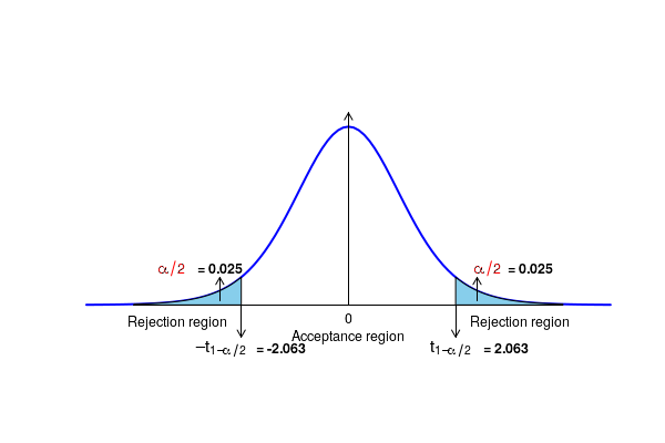
From the given data sets, we compute the mean and standard deviations: \(\small{\overline{X}=5.101 ,~~~S_X = 0.264,~~~~\overline{Y}= 4.733 ,~~~~S_Y= 0.307 ,~~~~with~~~n=10,~~m=12 }\) The statistic for the Welsch t test is computed as, \(\small{t_w = \dfrac{\overline{X} - \overline{Y}}{\sqrt{\dfrac{S_X^2}{n} + \dfrac{S_Y^2}{m}}}~~=~~= \dfrac{5.101 - 4.733 }{\sqrt{\dfrac{0.264^2}{10} + \dfrac{0.307^2}{12}}}~~=~~3.02 }\) The modified degrees of freeson r is computed using the Welsch-Satterthwaite correction formula as, \(~~~~\small{r = \dfrac{\left(\dfrac{s_X^2}{n} + \dfrac{s_Y^2}{m}\right)^2} {\dfrac{1}{n-1}\left(\dfrac{s_X^2}{n}\right)^2 + \dfrac{1}{m-1} \left(\dfrac{s_Y^2}{m}\right)^2}~~=~~\dfrac{\left(\dfrac{0.264^2}{10} + \dfrac{0.307^2}{10}\right)^2} {\dfrac{1}{10-1}\left(\dfrac{0.264^2}{10}\right)^2 + \dfrac{1}{12-1} \left(\dfrac{0.307^2}{12}\right)^2}~~=~~19.96 }\) We approximately take the degrees of freedom to the nearest integer to be $r=20$. Under the null hypotesis, the statistic $t_w$ follows t distribution with $r=20$ degrees of freedom. Testing null hypothesis using p value Since the null hypothesis $H_0 : \mu_X = \mu_Y$ can be rejected by higher and lower values of the distribution, this is a two sided test. With $\alpha=0.05$, we take $\alpha/2 = 0.025$ to be the significnce level on each side for testing the hypothesis. We compute the probability of getting a t statistic value above $t_w = 3.04$ in a t distribution with 24 degrees of freedom. From either t table or R function call "1 - pt(3.04, 20)" this is comuted to be 0.00323. Since this probability is less than the significance level 0.025, we reject the two sided null hypothesis to a significance level of 0.05. Testing null hypothesis using rejection regions For this two sided test, to a significant level of \(\small{\alpha=0.05 }\), we get, from t-tables, \(t_0 = t_{1-\alpha/2}(r) = t_{0.975}(20)= 2.086\) Since the computed value \(\small{t_w=3.02}\) of the t statistic is outside the range (\(\small{-t_0 \leq t \leq t_0) }\), we reject the null hypothesis and accept the alternate hypothesis to a significant level of \(\small{\alpha}\). Confidence interval for the difference in population means A $95\%$ confidence interval for the observed difference between population means is, \(\small{(\overline{X} - \overline{Y}) \pm t_{1-\alpha/2}(r) \sqrt{\dfrac{S_X^2}{n} + \dfrac{S_Y^2}{m} } ~=~(5.101 - 4.733) \pm 2.086 \sqrt{\dfrac{0.264^2}{10} + \dfrac{0.307^2}{12} } ~=~(0.114, 0.622) }\) Since this confidence interval does not contain 0 inside it, we reject the null and accept the alternate hypothesis.| Individual | $X_i$ | $Y_i$ | $d_i = X_i-Y_i$ | $d_i - \overline{d}$ | $(d_i - \overline{d})^2$ |
|---|---|---|---|---|---|
| 1 | 95 | 97 | -2 | 4.86 | 23.59 |
| 2 | 106 | 116 | -10 | -3.14 | 9.88 |
| 3 | 79 | 82 | -3 | 3.86 | 14.88 |
| 4 | 71 | 81 | -10 | -3.14 | 9.88 |
| 5 | 90 | 82 | 8 | 14.86 | 220.73 |
| 6 | 79 | 86 | -7 | -0.14 | 0.02 |
| 7 | 71 | 107 | -36 | -29.14 | 849.31 |
| 8 | 77 | 86 | -9 | -2.14 | 4.59 |
| 9 | 103 | 94 | 9 | 15.86 | 251.45 |
| 10 | 103 | 91 | 12 | 18.86 | 355.59 |
| 11 | 92 | 85 | 7 | 13.86 | 192.02 |
| 12 | 63 | 98 | -35 | -28.14 | 792.02 |
| 13 | 82 | 91 | -9 | -2.14 | 4.59 |
| 14 | 76 | 87 | -11 | -4.14 | 17.16 |

R-scripts
in R, the family of student's t-tets can be performed with a single call to the function
t.test(x, y, alternative, mu, paired, var.equal, conf.level) wherex, y = data vectors of two observationsalternative = A character string specifying alternate hypothesis. alternate can take three values :"two.sided", "less", "greater" It can also be a vector with all the above three strings, in which case all the three hypothesis will be tested. "less" means the population mean of x is less than that of y. "greater" mens the population mean of x is greater thn that of y. default value is"two.sided" mu = a number indicating the true value of the mean for one smple test, and the difference in the means in the case of two sample test.paired = A logical value ofTRUE orFALSE indicating whether it is a paired or unpaired test. Default isFALSE and hence an unpaired t testconf.level = confidence level of the interval. For example,conf.level=0.95 sets a 95% confidence interval. The function returns a vector with two numbers :(p value, Z statistics) .two_sample_Z_test(x, y, sigma_x, sigma_y, alpha, null) wherex, y = data vectors of two observationssigma_x, sigma_y = population standard deviationsalpha = significane levelnull = string value indicating type of null hypothesis. Possible values of variable null are:"equal", "less_than_or_equal", "more_than_or_equal" The function returns a data structure from which the p-value of the test and the confidence interval can be extracted along with other input values. Imortant Note : The p-value for a two sided test is the sum of p-values on bothe sides. See the R code example below for various tests with this function.## R script using t.test() library function for various t tests ##------------------------- Test-1 -------------------------------------------- ### Two sample t-test between two independent variables with unequal population variances ### This is "Welsch t-test" ##we set a confidence level of 0.95 # data sets Xvar=c(4.95,5.37,4.70,4.96,4.72,5.17,5.28,5.12,5.26,5.48) Yvar=c(4.65,4.86,4.57,4.56,4.96,4.63,5.04,4.92,5.37,4.58,4.26,4.40) ## The test is for a null hypothesis of equality of means. Alternate says that the means are ## unequal. Hence this is a two sided alternatie hypothesis . ## The difference between two population means is zero. ## call to the t.test() function res = t.test(x=Xvar, y=Yvar, alternative="two.sided", var.equal=FALSE, paired=FALSE, conf.level=0.95) ## Print the result summary print(res) ## Note : To perform a two smple independent t test with equality of variance, ## set "var.equal=TRUE" in the above function call print("------------------------------------------") ##----------------------------- Test-2 ----------------------------------------- ## Two sample t-test with dependent variables (paired t-test) data_before = c(95,106,79,71,90,79,71,77,103,103,92,63,82,76) data_after = c(97,116,82,81,82,86,107,86,94,91,85,98,91,87) ## we test the null hypothesis that the population means of 2 variables are equal ## to a significance level of 0.95 ## call to the t.test() function res = t.test(x=data_before, y=data_after, alternative="two.sided", paired=TRUE, conf.level=0.95) print(res) ##Executing the script in R prints the following lnes of test results:
Welch Two Sample t-test data: Xvar and Yvar t = 3.0216, df = 19.966, p-value = 0.006749 alternative hypothesis: true difference in means is not equal to 0 95 percent confidence interval: 0.1138185 0.6215148 sample estimates: mean of x mean of y 5.101000 4.733333 [1] "------------------------------------------" Paired t-test data: data_before and data_after t = -1.7654, df = 13, p-value = 0.101 alternative hypothesis: true difference in means is not equal to 0 95 percent confidence interval: -15.248261 1.533975 sample estimates: mean of the differences -6.857143