CountBio

Hypothesis testing a population proportion

We sometimes sample a population to estimate the proportion of the observations with favourable outcome which we call "success". For exmaple, a study aims to estimate the proportion of adult population in a city who use pain killers at least twice a month. A random sample of 1000 adults were asked this question and 79 of them answered that they take pain killers at least twice a month for some ailment or other. This gives a sample proportion \(~\small{p_s = \dfrac{79}{1000} = 0.079}\) for the favourable result.

The question is, how closely this proportion \(\small{p_s}\) observed in the sample data set reflects the corresponding proportion \(\small{p}\) in the entire poulation?.

For this, we test the null hypothesis that \(\small{p = p_0}\) against one of the three alternate hypothesis that \(\small{p \neq p_0,~p \gt p_0 ~and~ p \lt p_0 }\).

While studying the distribution followed by sample proportion, we have seen that the sample proportion \(\small{f}\) defines a Z staistic that follows a unit normal distribution:

\(\small{ Z~= \dfrac{p_s - p}{\sqrt{\dfrac{p(1-p)}{n} } } }~~~~\) approximately follows \(\small{N(0,1) }\) provided the sample size n is large.

How much n is large?

As a thumb rule, the formula for the Z statistic is valide only when sample size n is large enough, given by the condition \(\small{np_0 > 5}\) and \(\small{n(1-p_0) > 5 }\). For exmple, if $p_0 = 0.1$, then n should be at least 50.

We use this fact to test the null hypothesis that the proportion p in the population is equal to a particular value \(\small{p_0}\) against the three alternate hypothesis.

• Compute the sample proportion \(\small{p_s}\) from the data.


• For a given \(\small{p=p_0}\) and sample size n, compute the Z statistics using the above expression.


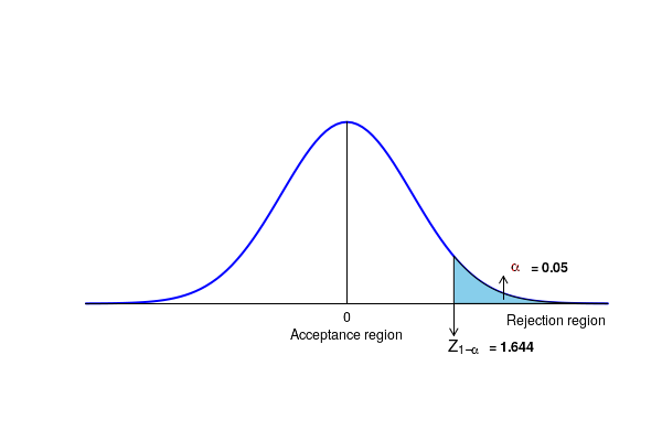
• For a given significance level of \(\small{\alpha}\), we reject the two sided null \(\small{H_0 : p = p_0 }\) and accept the two sided alternative \(\small{H_A : p \ne p_0 }\) if the computed Z value is outside the range \(\small{(-Z_{1-\alpha/2}, Z_{1-\alpha/2}) }\)
.
For an one sided alternative \(\small{H_A : p \gt p_0 }\), reject the null if \(\small{Z \gt Z_{1-\alpha} }\). Similarly, for an one sided alternative \(\small{H_A : p \lt p_0 }\), reject the null if \(\small{Z \lt -Z_{1-\alpha} }\)

Example-1 :

In an election to the member of parliment, a candidate lost the election by securing secured $14\%$ ofthe polled votes. Six months before the next election, his party conducted a regorous 3 months campaign to increase his support base among the voters. At the end of the campaign, an opinion poll was conducted among a randomly selected sample of 600 voters among whom 105 said that they would vote for him. Test whether there is a significant increase in his voter base. Use 0.05 as the significant level for the test.


Since we want to test whether the population fraction is significantly increased from 0.14, we set up the null and alternate hypothesis as follows:
\(~~~~~~~~~~~\small{H_0 : p\leq 0.14 } \)
\(~~~~~~~~~~~\small{H_A : p \gt 0.14}\)
Since the alternate hypothesis can be satisfied by the values greater than the given \(\small{p}\) value, this is a one sided test.

We first compute fraction of success in the sample. We get,
\(~~~~~~~~~\small{p_s = \dfrac{105}{600} = 0.175}\)

We compute the Z statistic from the data:

\(\small{Z~=~ \dfrac{p_s - p}{\sqrt{\dfrac{p(1-p)}{n} } } }\)

Under null hypothesis, the Z statistic should follow a unit normal distribution N(0,1). We compute the statistic from the data:

\(\small{ Z~= \dfrac{p_s - p}{\sqrt{\dfrac{p(1-p)}{n} } }~=~\dfrac{0.175 - 0.140}{\sqrt{\dfrac{0.175 (1-0.175)}{600}}}~=~2.256 }~~~~\)

testing the null hypothesis using rejection regions:

We have taken \(\small{\alpha =0.05}\) to be the probability for rejecting the null hypothesis. The critical value is \(\small{Z_{1-\alpha} = Z_{0.95} = 1.644 }\). Since this is a one sided test, the null hypothesis \(\small{H_0 : p \leq 0.140 }\) will be rejected by Z values greater than \(\small{1.644 }\)

This rejection region is indicated as shaded portion in the figure below:

Since the computed value Z = 2.256 is in the rejection region, we reject the null hypothesis to conclude that thefraction of population supporting the candidate is significantly higher than the previous value of 0.14. The statistical significance of this test is 0.05.

Testing the null hypothesis by computing the p-value for the observation:

For the computed Z value of 2.256, the p-value is obtained by computing the area under the unit normal curve to the right of this Zvalue. From the Gussian table or using the R command "1-pnorm(2.256)", we get this value as 0.012.

Since the p-value \(\small{p=0.012 }\) of the observed test statistic is less than \(\small{\alpha = 0.05}\), we reject the null hypothesis to a significance level of 0.05.

R-scripts

       binom.test(x, n, p, alternative) 

       prop.test(x, n, p, alternative, correct) 

where

       x  = number of successes

       n  = total number of trials
 
       p  = the proportion to test against

       alternative   = string value indicating type of null hypothesis. The three types are,

                                             "two.sided", "less", "greater". Default value is "two.sided".


       correct   = a logical "TRUE" or "FALSE" indicating whether "Yates correction" should be 
                                             applied where it is possible. Defailt value id TRUE.

      

The function returns a data structure with the results of the test.

##################################################
## One sample proportion test

## From a given adult population, a random sample of 2600 adult men were tested for obesity. 
## The data showed that 710 to be obese. From this data, can we conclude that more than 25 percent 
## of the population are obese? Let 0.05 be the significance level for this test.

##since the sample size is large, we use the binomial test.

x = 710

n = 2600

p = 0.25

alternative = "greater"

res =  binom.test(x, n, p, alternative)

print(res)

###############------------------------------------------------

Executing the above script in R prints the following results and figures of probability distribution on the screen:

	Exact binomial test

data:  710 and 2600
number of successes = 710, number of trials = 2600, p-value = 0.003766
alternative hypothesis: true probability of success is greater than 0.25
95 percent confidence interval:
 0.2587064 1.0000000
sample estimates:
probability of success 
             0.2730769