CountBio
Mathematical tools for natural sciences
Basic Statistics with R
Hypothesis testing the difference between two population proportions
We sometimes sample from two independent populations to estimate the proportion of their favourable outcomes. Let $n_1$ and $n_2$ be the random samples from two independent distributions. Let $Y_1$ and $Y_2$ be their respective favourable outcomes. From this we compute ther proportions \(\small{p_{s1} = \dfrac{Y_1}{n_1} }\) and \(\small{p_{s2} = \dfrac{Y_2}{n_2} }\) . If $p_1$ and $p_2$ are the proportions of favourable outcomes in the two populatons respectively, we can test the equlity of the parent population proportions using a test statistic created out of observed proportions. Here, we distinguish between two cases : one in which the sample sizes $n_1$ and $n_2$ are large, and the second case in which the samples sizes are small.
Z test for two proportions - when sample sizes are large
If $p_1$ and $p_2$ are the proportions of favourable outcomes in the two populatons respectively, the distribution of the difference in population proportions is given by,
\(\small{ \dfrac{\dfrac{Y_1}{n_1}- \dfrac{Y_2}{n_2}~-~(p_1-p_2)}{\sqrt{\dfrac{p_1(1-p_1)}{n_1} + \dfrac{p_2(1-p_2)}{n_2} } }~~~~~ }\) approximately will be \(\small{N(0,1)}\).
When we test the null hypothesis that $p_1 = p_2$, the appropriate statistic is given from the above expression by,
\(\small{Z = \dfrac{\dfrac{Y_1}{n_1}- \dfrac{Y_2}{n_2}}{\sqrt{\dfrac{p_1(1-p_1)}{n_1} + \dfrac{p_2(1-p_2)}{n_2} } }~~~~~ }\) approximately will be \(\small{N(0,1)}\).
If the sample sizes \(\small{n_1}\) and \(\small{n_2}\) are large enough, we can replace the probabilities \(\small{p_1}\) and \(\small{p_2}\) by their estimates \(\small{p_{s1}}\) and \(\small{p_{s2}}\) respectively in the denominator of the above expression. The test statistic becomes,
\(\small{Z = \dfrac{p_{s1}-p_{s2}}{\sqrt{\dfrac{p_{s1}(1-p_{s1})}{n_1} + \dfrac{p_{s2}(1-p_{s2})}{n_2} } }~~~~~ }\) approximately will be \(\small{N(0,1)}\).
We proceed with the hypothesis testing as follows:
- Compute the sample fractions \(\small{p_{s1}}\) and \(\small{p_{s2}}\) from the data.
- For the given sample sizes $n_1$ and $n_2$, compute the Z statistics using the above expression.
- For a given significance level of \(\small{\alpha}\), we reject the null \(\small{H_0 : p_1 = p_2 }\) and accept the two sided alternative \(\small{H_A : p_1 \ne p_2 }\) if the computed Z value is outside the range \(\small{(-Z_{1-\alpha/2}, Z_{1-\alpha/2}) }\). For an one sided alternative \(\small{H_A : p_1 \gt p_2 }\), reject the null if \(\small{Z \gt Z_{1-\alpha} }\). Similarly, for an one sided alternative \(\small{H_A : p_1 \lt p_2 }\), reject the null if \(\small{Z \lt -Z_{1-\alpha} }\)
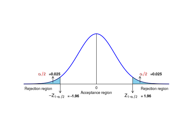
Since the computed value Z = -1.383 is in the acceptance region, we accept the null hypothesis to conclude that there is no significnce difference between the proportion of male and female students supporting the abolition of death penalty. The statistical significance of this test is 0.05.
Testing the null hypothesis by computing the p-value for the observation: For the computed Z value of -1.383, the p-value is obtained by computing the area under the unit normal curve to the right of this Zvalue. From the Gussian table or using the R command "pnorm(-1.383)", we get this value as 0.0833. Since the p-value \(\small{p=0.0833 }\) of the observed test statistic is greater than \(\small{\alpha = 0.025}\) for the two sided test, we accept the null hypothesis to a significance level of 0.05 to conclude that there is no significnce difference between the proportion of male and female students supporting the abolition of death penalty. Fisher's exact test for two proportions - when sample sizes are small
This test can be used even when the sample sizes are small. In this test, there are two populations X and Y. Among the $n_1$ random samples from X, there were $x_1$ favourable ourcomes. Smilarly, among the $n_2$ random samples from Y, favourble outcome was observed in $x_2$ samples. Let $n = n_1 + n_2$.
We rename the observation as,
\(\small{a = x_1,~~b = x_2,~~c = n_1-x_1,~~d = n_2 - x_2 ~~ }\) to write a $2 \times 2$ contingency table:
\(
\begin{array} {|r|r|}\hline & X & Y & Row~sum \\ \hline Favourable & a & b & a+b \\ \hline Not~favourable & c & d & c+d \\ \hline column~sum& a+c& b+d & a+b+c+d = n \\ \hline \end{array}
\)
For a given set of values for a,b,c and d, the probability of getting this table follows a hypergeometric distribution under the null hypothesis that the two distributions X and Y have equal fraction of favourable events:
\( \small{P_h(a,b,c,d,n) = \dfrac{\displaystyle \binom{a+b}{a} \binom{c+d}{c}}{\displaystyle \binom{n}{a+c}} = \dfrac{\displaystyle \binom{a+b}{b} \binom{c+d}{d}}{\displaystyle \binom{n}{b+d}} = \dfrac{(a+b)!(c+d)!(a+c)!(b+d)!}{a!b!c!d!n!} } \)
This expression gives th exact hypergeometric probability of observing this contingency table with particular valus of a,b,c,d under the null hypothesis that the two distributions contain equal fraction of favourable events. Since this probability is exactly computed without making approximations to larger sizes, it is called an exact test .
For computing the significance of observed data under null hypothesis, we compute the probability P(a,b,c,d,n) for various possible vlues of a,b,c and d while keeping the marginal totals (ie, row and column sums) same as the observed table. We then sum all these probabilities to see whether this total probability is less than the threshold value. This gives a one tailes test. For a two sided test, tables are contructed with extreme values in the opposite direction.
A very detailed description of this methdology can be found in the wikipedia page here.
R-scripts
In R, the function
prop.test(x, n, p= NULL, alternative = "two.sided", correct = TRUE) x = data vector of counts of successes.n = data vector containing number of trials in each case for which successes in x are observed.p = a vector of probabilities of successes.alternative = string value specifying alternate hypothesis. Possible values are "two.sided", "less" or "more"correct = A boolean value indicaing whether Yates continuity corretion to be applied. It is TRUE by default. The function returns a data structure with various results.
The Fisher's exact test can be perfored using the R library function
fisher.test(x, alternative = "two.sided", conf.int = TRUE, conf.level = 0.95) where,x is a 2 by 2 matrix contaning the values of the contingency table of events under categories. All other parameters are as defined before. This function can also perform test for contingency tables of dimension more than 2 by 2. Many more parameters are there. See "help(fisher.test") in R for more details.
##################################################
## Testing two population proportions with prop.test

## 1.  Using prop.test() functon

## In a health survey, 520 out of 600 men and 550 out of 600 women questioned said they use
## antibiotics whenever fever continues for more than 2 days. We want to test whether
## there is a significant difference in the fraction of men and women
## who start taking antibotics after 2 days of fever.

x = c(520, 550)  ## favourble response in each category of data

n = c(600, 600)  ## total samples in each category.

res = prop.test(x,n,alternative = "two.sided")

print(res)


#### Perform Fishers exact test for a contingency table.

## We have the following contingency table for patients belonging to two economic strata
## admitted for throat cancer in
## a hosital. They say whether they indulge in tobacco abuse or not:

##                    Higher-income      Lower-income
##
##  Tobacco abuse        11                17
##
##  No abuse             42                39
##

##We do Fishers exact test to find whether the patients from higher income group indulge in
## tobacco abuse in a significantly different proportion than the patients from
## lower income group

x = matrix(c(11,42,17,39), ncol=2)

res1 = fisher.test(x,  alternative = "two.sided",
		 conf.int = TRUE, conf.level = 0.95)

print(res1)


###############------------------------------------------------
Executing the above script in R prints the following results and figures of probability distribution on the screen:
	2-sample test for equality of proportions with continuity correction

data:  x out of n
X-squared = 7.2552, df = 1, p-value = 0.00707
alternative hypothesis: two.sided
95 percent confidence interval:
 -0.0867225 -0.0132775
sample estimates:
   prop 1    prop 2
0.8666667 0.9166667


	Fisher's Exact Test for Count Data

data:  x
p-value = 0.2797
alternative hypothesis: true odds ratio is not equal to 1
95 percent confidence interval:
 0.2250716 1.5641267
sample estimates:
odds ratio
 0.6036637